Bayesian Aggregation

Yang, Y., & Dunson, D. B., Minimax Optimal Bayesian Aggregation 2014 (arXiv)

Say we have a number of estimators \(\hat f_1, \ldots, \hat f_K\) derived from a number of models \(M_1, \ldots, M_K\) for some regression problem \(Y = f(X) + \epsilon\), but, as is the nature of things when estimating with limited data, we don’t know which estimator represents the true model (assuming the true model is in our list). The Bayesian habit is to stick a prior on the uncertainty, compute posteriors probabilities, and then average across the unknown parameter using the posterior probabilities as weights. Since the posterior probabilities (call them \(\lambda_1, \ldots, \lambda_K\)) have to sum to 1, we obtain a convex combination of our estimators \[ \hat f = \sum_{1\leq i \leq K} \lambda_i \hat f_i \] This is the approach of Bayesian Model Averaging (BMA). Yang et al. propose to find such combinations using a Dirichlet prior on the weights \(\lambda_i\). If we remove the restriction that the weights sum to 1 and instead only ask that they have finite sum in absolute value, then we obtain \(\hat f\) as a linear combination of \(\hat f_i\). The authors then place a Gamma prior on \(A = \sum_i |\lambda_i|\) and a Dirichlet prior on \(\mu_i = \frac{|\lambda_i|}{A}\). In both the linear and the convex cases they show that the resulting estimator is minimax optimal in the sense that it will give the best worst-case predictions for a given number of observations, including the case where a sparsity restriction is placed on the number of estimators \(\hat f_i\); in other words, \(\hat f\) converges to the true estimator as the number of observations increases with minimax optimal risk. The advantage to previous non-bayesian methods of linear or convex aggregation is that the sparsity parameter can be learned from the data. The Dirichlet convex combination gives good performance against Best Model selection, Majority Voting, and SuperLearner, especially when there are both a large number of observations and a large number of estimators.

I implemented the convex case in R for use with brms. The Dirichlet distribution has been reparameterized as a sum of Gamma RVs to aid in sampling. The Dirichlet concentration parameter is \(\frac{\alpha}{K^\gamma}\); the authors recommend choosing \(\alpha = 1\) and \(\gamma = 2\).

convex_regression <- function(formula, data,
                              family = "gaussian",
                              ## Yang (2014) recommends alpha = 1, gamma = 2
                              alpha = 1, gamma = 2,
                              verbose = 0,
                              ...) {
  if (gamma <= 1) {
    warning(paste("Parameter gamma should be greater than 1. Given:", gamma))
  }
  if (alpha <= 0) {
    warning(paste("Parameter alpha should be greater than 0. Given:", alpha))
  }
  ## Set up priors.
  K <- length(terms(formula))
  alpha_K <- alpha / (K^gamma)
  stanvars <-
    stanvar(alpha_K,
      "alpha_K",
      block = "data",
      scode = "  real<lower = 0> alpha_K;  // dirichlet parameter"
    ) +
    stanvar(
      name = "b_raw",
      block = "parameters",
      scode = "  vector<lower = 0>[K] b_raw; "
    ) +
    stanvar(
      name = "b",
      block = "tparameters",
      scode = "  vector[K] b = b_raw / sum(b_raw);"
    )
  prior <- prior("target += gamma_lpdf(b_raw | alpha_K, 1)",
    class = "b_raw", check = FALSE
  )
  f <- update.formula(formula, . ~ . - 1)
  if (verbose > 0) {
    make_stancode(f,
      prior = prior,
      data = data,
      stanvars = stanvars
    ) %>% message()
  }
  fit_dir <- brm(f,
    prior = prior,
    family = family,
    data = data,
    stanvars = stanvars,
    ...
  )
  fit_dir
}

Here is a gist that includes an interface to parsnip.

In my own experiments, I found the performance of the convex aggregator to be comparable to a LASSO SuperLearner at the cost of the lengthier training that goes with MCMC methods and the finicky convergence of sparse priors. So I would likely reserve this for when I had lots of features and lots of estimators to work through, where I presume it would show an advantage. But in that case it would definitely be on my list of things to try.

Bayesian Stacking

Yao, Y., Vehtari, A., Simpson, D., & Gelman, A., Using Stacking to Average Bayesian Predictive Distributions (pdf)

Another approach to model combination is stacking. With stacking, model weights are chosen by cross-validation to minimize RMSE predictive error. Now, BMA finds the aggregated model that best fits the data, while stacking finds the aggregated model that gives the best predictions. Stacking therefore is usually better when predictions are what you want. A drawback is that stacking produces models through point estimates. So, they don’t give you all the information of a full distribution like BMA would. Yao et al. propose a method of stacking that instead finds the optimal predictive distribution by convex combinations of distributions with weights chosen by some scoring rule: the authors use the minimization of KL-divergence. Hence, they choose weights \(w\) empirically through LOO by \[ \max_w \frac{1}{n} \sum_{1\leq i \leq n} \log \sum_{1\leq k \leq K} w_k p(y_i | y_{-i}, M_k) \] where \(y_1, \ldots, y_n\) are the observed data and \(y_{-i}\) is the data with \(y_i\) left out. The following figure shows how stacking of predictive distributions gives the “best of both worlds” for BMA and point prediction stacking.

From Yao (2018)
From Yao (2018)

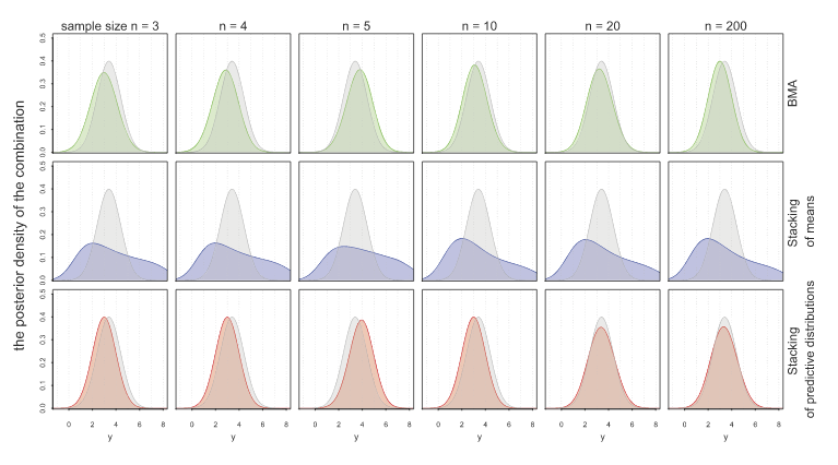
They have implemented stacking for Stan models in the R package loo.

I wrote a little package recently for a project I’ve been working on. I’ve mostly been using it to help out with Monte Carlo simulations for personal finance planning. It’s a little rough at the moment, but for the adventurous it’s on Github here: investmentsim. And here’s a quick tutorial on how to use it.

The investmentsim package implements a function make_path to simulate an investment portfolio. It supports time-varying allocation of assets, automatic rebalancing, and planned transactions. The purpose of the package is to backtest investment plans as one might do for retirement accounts. (It does not have support for taxes or fees.)

This example will demonstrate how to create an investment portfolio with defined allocations and transactions, and then simulate the balance of the portfolio over a period of time.

library(tidyverse)
library(xts)
library(lubridate)
library(investmentsim)

First let’s create a portfolio. The simreturns data contains an xts time-series with fictional yearly returns for a stock fund and a bond fund over the years 1928 to 2018.

data(simreturns)
head(simreturns)
#>            Stock.Returns Bond.Returns
#> 1928-01-01    0.11867241   0.01866146
#> 1929-01-01    0.04008497   0.02362385
#> 1930-01-01    0.16592113   0.04912787
#> 1931-01-01    0.18508859  -0.03370055
#> 1932-01-01    0.05509245   0.06772749
#> 1933-01-01    0.07558251   0.04195868

An asset in the investmentsim package is a function with parameters start and end that returns the percent change in the asset over the dates from start to end. The make_historical function will construct an asset given a time-series of returns. This function is supposed to be used when you want to use predetermined data as opposed to something generated at runtime.

simstock_asset <- make_historical(simreturns$Stock.Returns)
simbond_asset <- make_historical(simreturns$Bond.Returns)

Next we define a portfolio with the make_portfolio function. It takes a list of names for the assets together with the functions defining them and a list for their initial balances. Also, let’s define a sequences of dates over which we’ll run the simulation.

asset_names <- c("Stocks", "Bonds")
port <- make_portfolio(asset_names,
                       c(simstock_asset,
                         simbond_asset),
                       c(2500, 2500))
dates <- seq(ymd("1940-01-01"), ymd("2010-01-01"), by="years")

Then we can define our desired allocations with make_linear_allocation. It needs a list of dates and also a list of percentages for each asset.

alloc <- make_linear_allocation_path(asset_names,
                                     c(ymd("1970-01-01"),
                                       ymd("2000-01-01")),
                                     list(c(0.9, 0.1),
                                          c(0.4, 0.6)))

It’s easiest to see how it works by looking at a graph.

as <- map(dates,
          alloc) %>%
    do.call(rbind, .) %>%
    xts(order.by = dates)

plot(as, ylim = c(0, 1),
     col = c("red", "blue"),
     main = "Asset Allocation")
addLegend("topright",
          asset_names,
          col = c("red", "blue"),
          lty = 1, cex = 1,
          bty = "o")
The allocation path for the portfolio.

You can see that it is constant before the first date given and constant after the last date, and that it linearly interpolates the allocation when moving from one date to the next.

Finally, we can define our desired transactions and collect everything together in a model. The make_transactions_on_dates function does what it sounds like it does: defines for the model a specified deposit (a positive value) or a specified withdrawal (a negative value). Within the simulation, transactions are applied at the end of the years given. So this transaction path just makes a $1000 deposit at the end of each year.

trans <- make_transactions_on_dates(rep(1000, length(dates)),
                                    dates)
model <- make_model(port, alloc, trans, dates)

Lastly, we evaluate make_path on the model to run the simulation.

path <- make_path(model)
c(head(path), tail(path))
#>                  Stocks        Bonds        Total Transaction
#> 1940-01-01     2500.000 2.500000e+03     5000.000           0
#> 1941-01-01     6090.672 6.767413e+02     6767.413        1000
#> 1942-01-01     7606.609 8.451788e+02     8451.788        1000
#> 1943-01-01     7997.775 8.886416e+02     8886.416        1000
#> 1944-01-01    11848.487 1.316499e+03    13164.986        1000
#> 1945-01-01    13939.015 1.548779e+03    15487.794        1000
#> 2005-01-01 11137858.729 1.670679e+07 27844646.822        1000
#> 2006-01-01 12831289.074 1.924693e+07 32078222.685        1000
#> 2007-01-01 14673102.513 2.200965e+07 36682756.282        1000
#> 2008-01-01 16844539.341 2.526681e+07 42111348.352        1000
#> 2009-01-01 16949487.079 2.542423e+07 42373717.697        1000
#> 2010-01-01 20340375.373 3.051056e+07 50850938.433        1000
plot(path[,1:3],
     col = c("red", "blue", "green"),
     main = "Investment Path")
addLegend("topleft",
          c(asset_names, "Total"),
          col = c("red", "blue", "green"),
          lty = 1, cex = 1,
          bty = "o")
The value of the portfolio over time.

We’re rich!