Introduction

What are eigenvalues? What are singular values? They both describe the behavior of a matrix on a certain set of vectors. The difference is this: The eigenvectors of a matrix describe the directions of its invariant action. The singular vectors of a matrix describe the directions of its maximum action. And the corresponding eigen- and singular values describe the magnitude of that action.

They are defined this way. A scalar \(\lambda\) is an eigenvalue of a linear transformation \(A\) if there is a vector \(v\) such that \(A v = \lambda v\), and \(v\) is called an eigenvector of \(\lambda\). A scalar \(\sigma\) is a singular value of \(A\) if there are (unit) vectors \(u\) and \(v\) such that \(A v = \sigma u\) and \(A^* u = \sigma v\), where \(A^*\) is the conjugate transpose of \(A\); the vectors \(u\) and \(v\) are singular vectors. The vector \(u\) is called a left singular vector and \(v\) a right singular vector.

Eigenvalues and Eigenvectors

That eigenvectors give the directions of invariant action is obvious from the definition. The definition says that when \(A\) acts on an eigenvector, it just multiplies it by a constant, the corresponding eigenvalue. In other words, when a linear transformation acts on one of its eigenvectors, it shrinks the vector or stretches it and reverses its direction if \(\lambda\) is negative, but never changes the direction otherwise. The action is invariant.

Take this matrix, for instance:

\[ A = \begin{bmatrix} 0 & 2 \\ 2 & 0 \end{bmatrix} \]

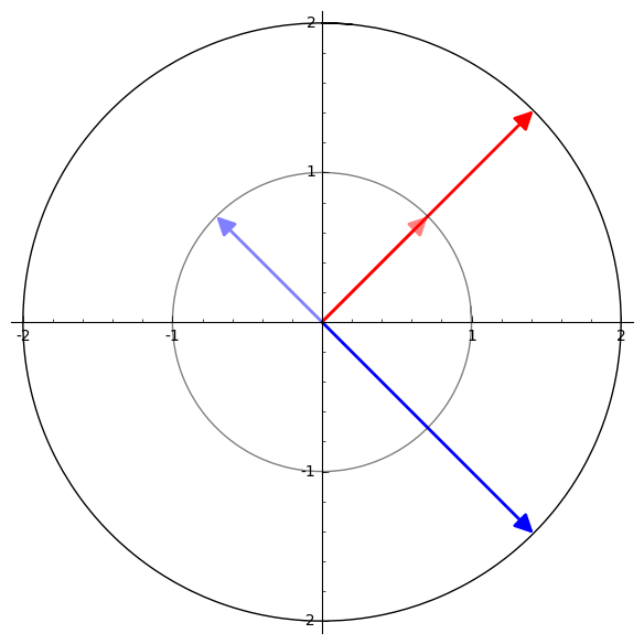
We can see how the transformation just stretches the red vector by a factor of 2, while the blue vector it stretches but also reflects over the origin.

And this matrix:

\[ A = \begin{bmatrix} 1 & \frac{1}{3} \\ \frac{4}{3} & 1 \end{bmatrix} \]

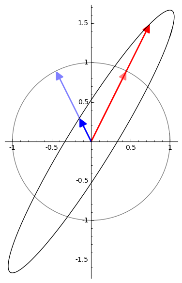
It stretches the red vector and shrinks the blue vector, but reverses neither.

The point is that in every case, when a matrix acts on one of its eigenvectors, the action is always in a parallel direction.

Singular Values and Singular Vectors

This invariant direction does not necessarily give the transformation’s direction of greatest effect, however. You can see that in the previous example. But say \(\sigma_1\) is the largest singular value of \(A\) with right singular vector \(v\). Then \(v\) is a solution to

\[ \operatorname*{argmax}_{x, ||x||=1} ||A x|| \]

In other words, \( ||A v|| = \sigma_1 \) is at least as big as \( ||A x|| \) for any other unit vector \(x\). It’s not necessarily the case that \(A v\) is parallel to \(v\), though.

Compare the eigenvectors of the matrix in the last example to its singular vectors:

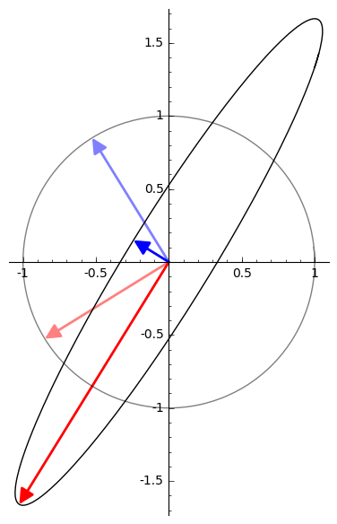
The directions of maximum effect will be exactly the semi-axes of the ellipse, the ellipse which is the image of the unit circle under \(A\).

Let’s extend this idea to 3-dimensional space to get a better idea of what’s going on. Consider this transformation:

\[A = \begin{bmatrix} \frac{3}{2} \, \sqrt{2} & -\sqrt{2} & 0 \\ \frac{3}{2} \, \sqrt{2} & \sqrt{2} & 0 \\ 0 & 0 & 1 \end{bmatrix} \]

This will have the effect of transforming the unit sphere into an ellipsoid:

Its singular values are 3, 2, and 1. You can see how they again form the semi-axes of the resulting figure.

Matrix Approximation with SVD

Now, the singular value decomposition (SVD) will tell us what \(A\)’s singular values are:

\[ A = U \Sigma V^* = \begin{bmatrix} \frac{\sqrt{2}}{2} & -\frac{\sqrt{2}}{2} & 0.0 \\ \frac{\sqrt{2}}{2} & \frac{\sqrt{2}}{2} & 0.0 \\ 0 & 0 & 1 \end{bmatrix} \begin{bmatrix} 3 & 0 & 0 \\ 0 & 2 & 0 \\ 0 & 0 & 1 \end{bmatrix} \begin{bmatrix} 1 & 0 & 0 \\ 0 & 1 & 0 \\ 0 & 0 & 1 \end{bmatrix} \]

The diagonal entries of the matrix \(\Sigma\) are the singular values of \(A\). We can obtain a lower-dimensional approximation to \(A\) by setting one or more of its singular values to 0.

For instance, say we set the largest singular value, 3, to 0. We then get this matrix:

\[ A_1 = \begin{bmatrix} \frac{\sqrt{2}}{2} & -\frac{\sqrt{2}}{2} & 0.0 \\ \frac{\sqrt{2}}{2} & \frac{\sqrt{2}}{2} & 0.0 \\ 0 & 0 & 1 \end{bmatrix} \begin{bmatrix} 0 & 0 & 0 \\ 0 & 2 & 0 \\ 0 & 0 & 1 \end{bmatrix} \begin{bmatrix} 1 & 0 & 0 \\ 0 & 1 & 0 \\ 0 & 0 & 1 \end{bmatrix} = \begin{bmatrix} 0 & -\frac{\sqrt{2}}{2} & 0 \\ 0 & \frac{\sqrt{2}}{2} & 0 \\ 0 & 0 & 1 \end{bmatrix} \]

which transforms the unit sphere like this:

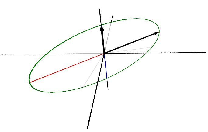
The resulting figure now lives in a 2-dimensional space. Further, the largest singular value of \(A_1\) is now 2. Set it to 0:

\[ A_2 = \begin{bmatrix} \frac{\sqrt{2}}{2} & -\frac{\sqrt{2}}{2} & 0.0 \\ \frac{\sqrt{2}}{2} & \frac{\sqrt{2}}{2} & 0.0 \\ 0 & 0 & 1 \end{bmatrix} \begin{bmatrix} 0 & 0 & 0 \\ 0 & 0 & 0 \\ 0 & 0 & 1 \end{bmatrix} \begin{bmatrix} 1 & 0 & 0 \\ 0 & 1 & 0 \\ 0 & 0 & 1 \end{bmatrix} = \begin{bmatrix} 0 & 0 & 0 \\ 0 & 0 & 0 \\ 0 & 0 & 1 \end{bmatrix} \]

And we get a 1-dimensional figure, and a final largest singular value of 1:

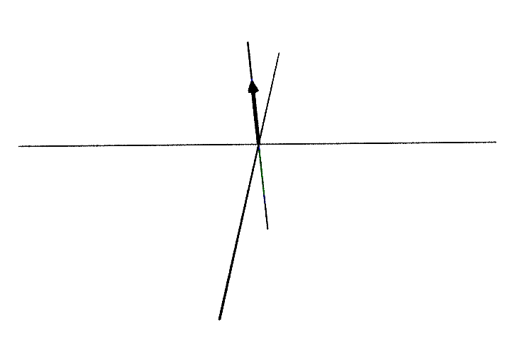
This is the point: Each set of singular vectors will form an orthonormal basis for some linear subspace of \(\mathbb{R}^n\). A singular value and its singular vectors give the direction of maximum action among all directions orthogonal to the singular vectors of any larger singular value.

This has important applications. There are many problems in statistics and machine learning that come down to finding a low-rank approximation to some matrix at hand. Principal component analysis is a problem of this kind. It says: approximate some matrix \(X\) of observations with a number of its uncorrelated components of maximum variance. This problem is solved by computing its singular value decomposition and setting some of its smallest singular values to 0.