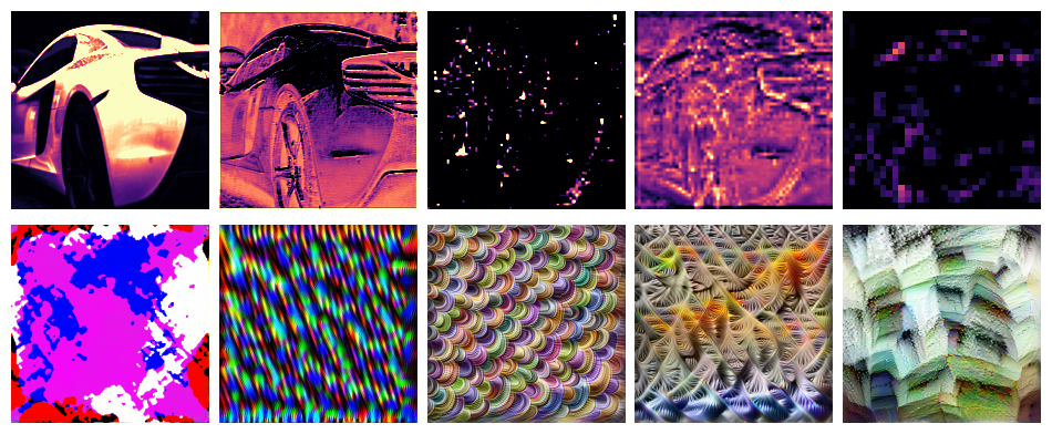
Convolutional neural networks (or convnets) create task-relevant representations of the training images by learning filters, which isolate from an image some feature of interest. Trained to classify images of cars, for example, a convnet might learn to filter for certain body or tire shapes.

In this article we’ll look at a couple ways of visualizing the filters a convnet creates during training and what kinds of features these correspond to in the training data. The first method is to look at the feature maps or (activation maps) a filter produces, which show us roughly where in an image the filter detected some feature. The second way will be through optimization visuzalizations, where we create an image of a filter’s preferred feature type through gradient optimization.

Such visualizations illustrate the process of deep learning. Through deep stacks of convolutional layers, a convnet can learns to recognize a complex hierarchy of features. At each layer, features combine and recombine features from previous layers, becoming more complex and refined.

We’ll outline the two techniques here, but you can find the complete Python implementation on Github.

The Activation Model

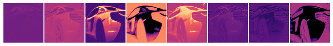
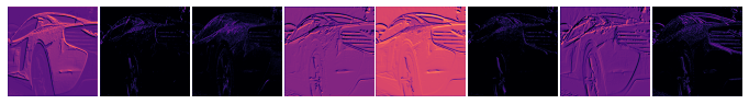
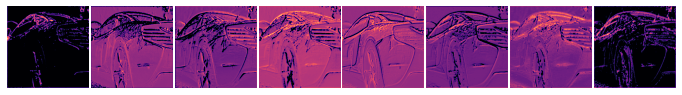
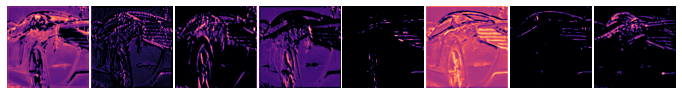
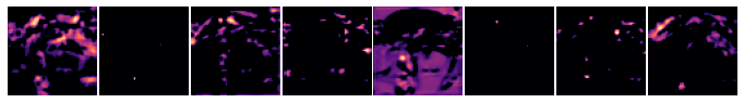
Each filter in a convolutional layer generally produces an output of shape [height, width]. These outputs are stacked depthwise by the layer to produce [height, width, channel], one channel per filter. So a feature map is just one channel of a convolutional layer’s output. To look at feature maps, we’ll create an activation model, essentially by rerouting the output produced by a filter into a new model.

import tensorflow as tf
from tensorflow import keras
from tensorflow.keras.applications import VGG16


def make_activation_model(model, layer_name, filter):
    layer = model.get_layer(layer_name)  # Grab the layer
    feature_map = layer.output[:, :, :, filter]  # Get output for the given filter
    activation_model = keras.Model(
        inputs=model.inputs,  # New inputs are original inputs (images)
        outputs=feature_map,  # New outputs are the filter's outputs (feature maps)
    )
    return activation_model


def show_feature_map(image, model, layer_name, filter, ax=None):
    act = make_activation_model(model, layer_name, filter)
    feature_map = tf.squeeze(act(tf.expand_dims(image, axis=0)))
    if ax is None:
        fig, ax = plt.subplots()
    ax.imshow(
        feature_map, cmap="magma", vmin=0.0, vmax=1.0,
    )
    return ax


# Use like:
# show_feature_map(image, vgg16, "block4_conv1", filter=0)

Here is a sample of the first few feature maps from layers in VGG16:

Optimization Visualization

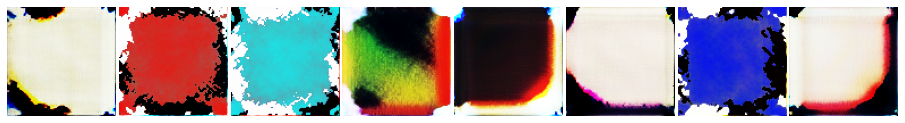
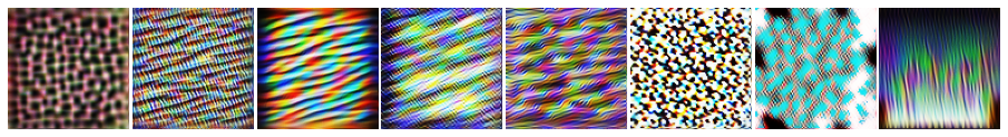
What kind of feature will activate a given filter the most? We can find out by optimizing a random image through gradient ascent. We’ll use the filter’s activation model like before and train the image pixels just like we’d train the weights of a neural network.

Here’s a simple Keras-style implementation:

class OptVis:
    def __init__(
        self, model, layer, filter, size=[128, 128],
    ):
        # Activation model
        activations = model.get_layer(layer).output
        activations = activations[:, :, :, filter]
        self.activation_model = keras.Model(
            inputs=model.inputs, outputs=activations
        )
        # Random initialization image
        self.shape = [1, *size, 3]
        self.image = tf.random.uniform(shape=self.shape, dtype=tf.float32)

    def __call__(self):
        image = self.activation_model(self.image)
        return image

    def compile(self, optimizer):
        self.optimizer = optimizer

    @tf.function
    def train_step(self):
        # Compute loss
        with tf.GradientTape() as tape:
            image = self.image
            # We can include here various image parameterizations to
            # improve the optimization here. The complete code has:
            #
            # - Color decorrelation on Imagenet statistics
            # - Spatial decorrelation through a Fourier-space transform
            # - Random affine transforms: jitter, scale, rotate
            # - Gradient clipping
            #
            # These greatly improve the result
            #
            # The "loss" in this case is the mean activation produced
            # by the image
            loss = tf.math.reduce_mean(self.activation_model(image))
        # Apply *negative* gradient, because want *maximum* activation
        grads = tape.gradient(loss, self.image)
        self.optimizer.apply_gradients([(-grads, self.image)])
        return {"loss": loss}

    @tf.function
    def fit(self, epochs=1, log=False):
        for epoch in tf.range(epochs):
            loss = self.train_step()
            if log:
                print("Score: {}".format(loss["loss"]))
        image = self.image
        return to_valid_rgb(image)

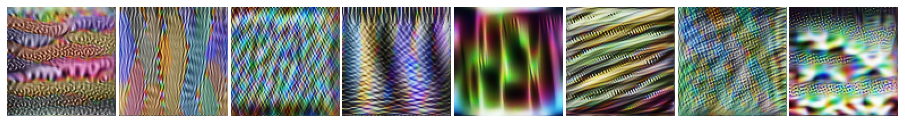
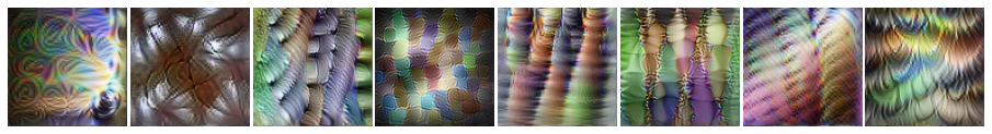
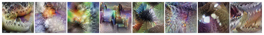
Here is a sample from ResNet50V2: