I wrote a little package recently for a project I’ve been working on. I’ve mostly been using it to help out with Monte Carlo simulations for personal finance planning. It’s a little rough at the moment, but for the adventurous it’s on Github here: investmentsim. And here’s a quick tutorial on how to use it.

The investmentsim package implements a function make_path to simulate an investment portfolio. It supports time-varying allocation of assets, automatic rebalancing, and planned transactions. The purpose of the package is to backtest investment plans as one might do for retirement accounts. (It does not have support for taxes or fees.)

This example will demonstrate how to create an investment portfolio with defined allocations and transactions, and then simulate the balance of the portfolio over a period of time.

library(tidyverse)
library(xts)
library(lubridate)
library(investmentsim)

First let’s create a portfolio. The simreturns data contains an xts time-series with fictional yearly returns for a stock fund and a bond fund over the years 1928 to 2018.

data(simreturns)
head(simreturns)
#>            Stock.Returns Bond.Returns
#> 1928-01-01    0.11867241   0.01866146
#> 1929-01-01    0.04008497   0.02362385
#> 1930-01-01    0.16592113   0.04912787
#> 1931-01-01    0.18508859  -0.03370055
#> 1932-01-01    0.05509245   0.06772749
#> 1933-01-01    0.07558251   0.04195868

An asset in the investmentsim package is a function with parameters start and end that returns the percent change in the asset over the dates from start to end. The make_historical function will construct an asset given a time-series of returns. This function is supposed to be used when you want to use predetermined data as opposed to something generated at runtime.

simstock_asset <- make_historical(simreturns$Stock.Returns)
simbond_asset <- make_historical(simreturns$Bond.Returns)

Next we define a portfolio with the make_portfolio function. It takes a list of names for the assets together with the functions defining them and a list for their initial balances. Also, let’s define a sequences of dates over which we’ll run the simulation.

asset_names <- c("Stocks", "Bonds")
port <- make_portfolio(asset_names,
                       c(simstock_asset,
                         simbond_asset),
                       c(2500, 2500))
dates <- seq(ymd("1940-01-01"), ymd("2010-01-01"), by="years")

Then we can define our desired allocations with make_linear_allocation. It needs a list of dates and also a list of percentages for each asset.

alloc <- make_linear_allocation_path(asset_names,
                                     c(ymd("1970-01-01"),
                                       ymd("2000-01-01")),
                                     list(c(0.9, 0.1),
                                          c(0.4, 0.6)))

It’s easiest to see how it works by looking at a graph.

as <- map(dates,
          alloc) %>%
    do.call(rbind, .) %>%
    xts(order.by = dates)

plot(as, ylim = c(0, 1),
     col = c("red", "blue"),
     main = "Asset Allocation")
addLegend("topright",
          asset_names,
          col = c("red", "blue"),
          lty = 1, cex = 1,
          bty = "o")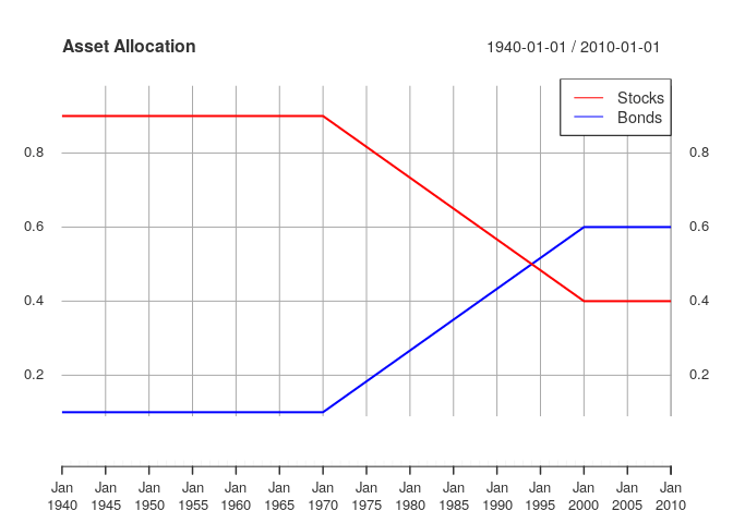

You can see that it is constant before the first date given and constant after the last date, and that it linearly interpolates the allocation when moving from one date to the next.

Finally, we can define our desired transactions and collect everything together in a model. The make_transactions_on_dates function does what it sounds like it does: defines for the model a specified deposit (a positive value) or a specified withdrawal (a negative value). Within the simulation, transactions are applied at the end of the years given. So this transaction path just makes a $1000 deposit at the end of each year.

trans <- make_transactions_on_dates(rep(1000, length(dates)),
                                    dates)
model <- make_model(port, alloc, trans, dates)

Lastly, we evaluate make_path on the model to run the simulation.

path <- make_path(model)
c(head(path), tail(path))
#>                  Stocks        Bonds        Total Transaction
#> 1940-01-01     2500.000 2.500000e+03     5000.000           0
#> 1941-01-01     6090.672 6.767413e+02     6767.413        1000
#> 1942-01-01     7606.609 8.451788e+02     8451.788        1000
#> 1943-01-01     7997.775 8.886416e+02     8886.416        1000
#> 1944-01-01    11848.487 1.316499e+03    13164.986        1000
#> 1945-01-01    13939.015 1.548779e+03    15487.794        1000
#> 2005-01-01 11137858.729 1.670679e+07 27844646.822        1000
#> 2006-01-01 12831289.074 1.924693e+07 32078222.685        1000
#> 2007-01-01 14673102.513 2.200965e+07 36682756.282        1000
#> 2008-01-01 16844539.341 2.526681e+07 42111348.352        1000
#> 2009-01-01 16949487.079 2.542423e+07 42373717.697        1000
#> 2010-01-01 20340375.373 3.051056e+07 50850938.433        1000

plot(path[,1:3],
     col = c("red", "blue", "green"),
     main = "Investment Path")
addLegend("topleft",
          c(asset_names, "Total"),
          col = c("red", "blue", "green"),
          lty = 1, cex = 1,
          bty = "o")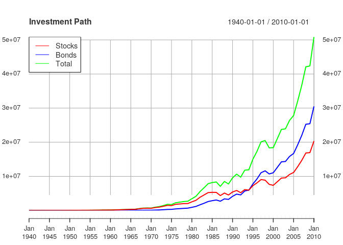

We’re rich!