Introduction

Say \(V\) and \(W\) are vector spaces with scalars in some field \(\mathbb{F}\) (the real numbers, maybe). A linear map is a function \(T : V \rightarrow W \) satisfying two conditions:

• additivity \(T(x + y) = T x + T y\) for all \(x, y \in V\)
• homogeneity \(T(c x) = c (T x)\) for all \(c \in \mathbb{F} \) and all \(x \in V\)

Defining a linear map this way just ensures that anything that acts like a vector in \(V\) also acts like a vector in \(W\) after you map it over. It means that the map preserves all the structure of a vector space after it’s applied.

It’s a simple definition – which is good – but doesn’t speak much to the imagination. Since linear algebra is possibly the most useful and most ubiquitous of all the branches of mathematics, we’d like to have some intuition about what linear maps are so we have some idea of what we’re doing when we use it. Though not all vectors live there, the Euclidean plane \(\mathbb{R}^2\) is certainly the easiest to visualize, and the way we measure distance there is very similar to the way we measure error in statistics, so we can feel that our intuitions will carry over.

It turns out that all linear maps in \(\mathbb{R}^2\) can be factored into just a few primitive geometric operations: scaling, rotation, and reflection. This isn’t the only way to factor these maps, but I think it’s the easiest to understand. (We could get by without rotations, in fact.)

Three Primitive Transformations

Scaling

A (non-uniform) scaling transformation \(D\) in \(\mathbb{R}^2\) is given by a diagonal matrix:

\[Scl(d1, d2) = \begin{bmatrix} d_1 & 0 \\ 0 & d_2 \\ \end{bmatrix}\]

where \(d_1\) and \(d_2\) are non-negative. The transformation has the effect of stretching or shrinking a vector along each coordinate axis, and, so long as \(d_1\) and \(d_2\) are positive, it will also preserve the orientation of vectors after mapping because in this case \(\det(D) = d_1 d_2 > 0\).

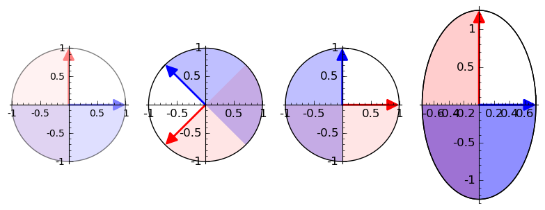
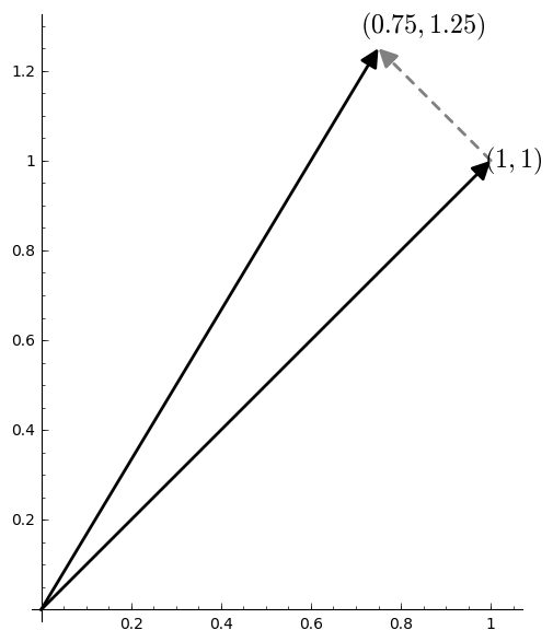
For instance, here is the effect on a vector of this matrix: \[D = \begin{bmatrix} 0.75 & 0 \\ 0 & 1.25 \\ \end{bmatrix}\]

It will shrink a vector by a factor of 0.75 along the x-axis and stretch a vector by a factor of 1.25 along the y-axis.

If we think about all the vectors of length 1 as being the points of the unit circle, then we can get an idea of how the transformation will affect any vector. We can see a scaling as a continous transformation beginning at the identity matrix.

If one of the diagonal entries is 0, then it will collapse the circle on the other axis.

\[D = \begin{bmatrix} 0 & 0 \\ 0 & 1.25 \\ \end{bmatrix}\]

This is an example of a rank-deficient matrix. It maps every vector onto the y-axis, and so its image has a dimension less than the dimension of the full space.

Rotation

A rotation transformation \(Ref\) is given by a matrix: \[Ref(\theta) = \begin{bmatrix} \cos(\theta) & -\sin(\theta) \\ \sin(\theta) & \cos(\theta) \\ \end{bmatrix}\]

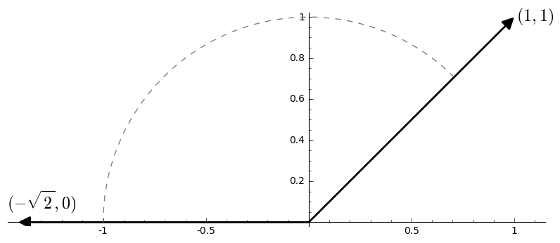
This transformation will have the effect of rotating a vector counter-clockwise by an angle \(\theta\), when \(\theta\) is positive, and clockwise by \(\theta\) when \(\theta\) is negative.

And the unit circle gets mapped onto itself.

It shouldn’t be too hard to convince ourselves that the matrix we’ve written down is the one we want. Take some unit vector and write its coordinates like \((\cos\gamma, \sin\gamma)\). Multiply it by \(Ref(\theta)\) to get \((\cos\gamma \cos\theta - \sin\gamma \sin\theta, \cos\gamma \sin\theta + \sin\gamma \cos\theta)\). But by a trigonometric identity, this is exactly the vector \((\cos(\gamma + \theta), \sin(\gamma + \theta))\), which is our vector rotated by \(\theta\).

A rotation should preserve not only orientations, but also distances. Now, recall that the determinant for a \(2\times 2\) matrix \(\begin{bmatrix} a & b \\ c & d \end{bmatrix}\) is \(a d - b c\). So a rotation matrix will have determinant \(\cos^2(\theta) + \sin^2(\theta)\), which, by the Pythagorean identity, is equal to 1. This, together with the fact that its columns are orthonormal means that it does preserve both. It is a kind of orthogonal matrix, which is a kind of isometry.

Reflection

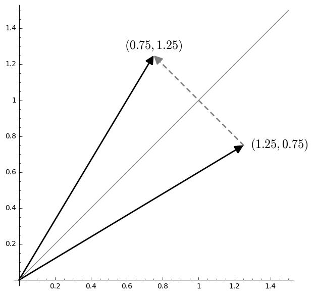
A reflection in \(\mathbb{R}^2\) can be described with matricies like: \[Ref(\theta) = \begin{bmatrix} \cos(2\theta) & \sin(2\theta) \\ \sin(2\theta) & -\cos(2\theta) \\ \end{bmatrix}\] where the reflection is through a line crossing the origin and forming an angle \(\theta\) with the x-axis.

And the unit circle gets mapped onto itself.

Note that the determinant of this matrix is -1, which means that it reverses orientation. But its columns are still orthonormal, and so it too is an isometry.

Decomposing Matricies into Primitives

The singular value decomposition (SVD) will factor any matrix \(A\) having like this:

\[ A = U \Sigma V^* \]

We are working with real matricies, so \(U\) and \(V\) will both be orthogonal matrices. This means each of these will be either a reflection or a rotation, depending on the pattern of signs in its entries. The matrix \(\Sigma\) is a diagonal matrix with non-negative entries, which means that it is a scaling transform. (The \(*\) on the \(V\) is the conjugate-transpose operator, which just means ordinary transpose when \(V\) doesn’t contain any imaginary entries. So, for us, \(V^* = V^\top\).) Now with the SVD we can rewrite any linear transformation as:

1. \(V^*\): Rotate/Reflect
2. \(\Sigma\): Scale
3. \(U\): Rotate/Reflect

Example

\[\begin{bmatrix} 0.5 & 1.5 \\ 1.5 & 0.5 \end{bmatrix} \approx \begin{bmatrix} -0.707 & -0.707 \\ -0.707 & 0.707 \end{bmatrix} \begin{bmatrix} 2.0 & 0.0 \\ 0.0 & 1.0 \end{bmatrix} \begin{bmatrix} -0.707 & -0.707 \\ 0.707 & -0.707 \end{bmatrix} \]

This turns out to be:

1. \(V^*\): Rotate clockwise by \(\theta = \frac{3 \pi}{4}\).
2. \(\Sigma\): Scale x-coordinate by \(d_1 = 2\) and y-coordinate by \(d_2 = 1\).
3. \(U\): Reflect over the line with angle \(-\frac{3\pi}{8}\).

Example

And here is a shear transform, represented as: rotation, scale, rotation.