Introduction

Gaussian Discriminant Analysis (GDA) is the name for a family of classifiers that includes the well-known linear and quadratic classifiers. These classifiers use class-conditional normal distributions as the data model for their observed features:

\[(X \mid C = c) \sim Normal(\mu_c, \Sigma_c) \]

As we saw in the post on optimal decision boundaries, the classification problem is solved by maximizing the posterior probability of class \(C=c\) given the observed data \(X\). From Bayes’ theorem, the addition of class distributions to our model then determines the problem completely:

\[ p(C = c \mid X) = \frac{p(X \mid C = c)p(C=c)}{\Sigma_{c'} p(X \mid C = c')p(C=c')} \]

A typical set of class-conditional distributions for a binary classification problem might look like this:

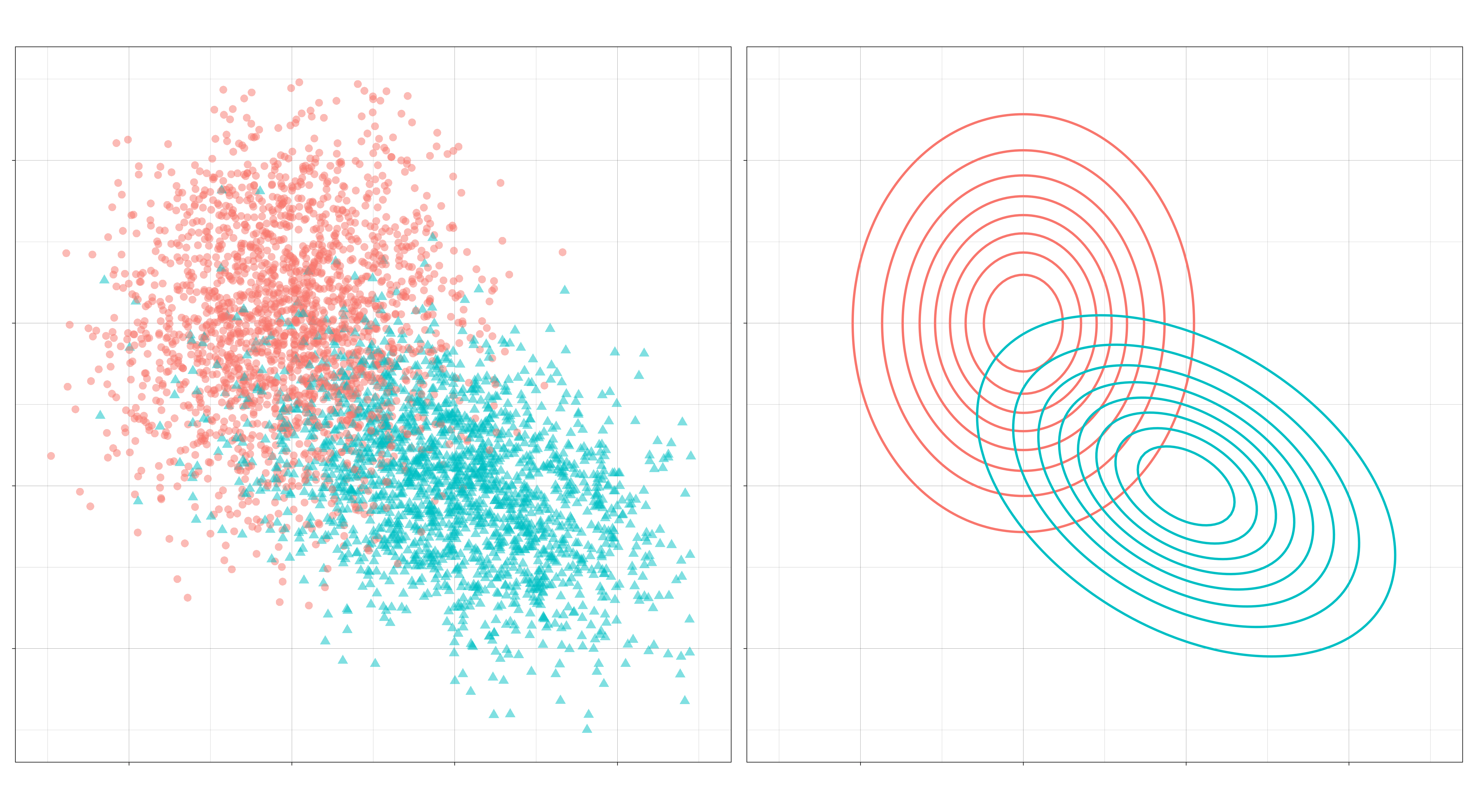
The classification problem then is to draw a boundary that optimally separates the two distributions.

Typically, this boundary is formed by comparing discriminant functions, obtained by plugging in normal densities into the Bayes’ formula above. For a given observation, these discriminant functions assign a score to each class; the class with the highest score is the class chosen for that observation.

In the most general case, the discriminant function looks like this:

\[ \delta_c(x) = -\frac{1}{2} \log \lvert\Sigma_c\rvert - \frac{1}{2}(x-\mu_c)^\top \Sigma_c^{-1}(x-\mu_c) + \log \pi_c \]

where \(\pi_c = p(C = c)\) is the prior probability of class \(c\). The optimal decision boundary is formed where the contours of the class-conditional densities intersect – because this is where the classes’ discriminant functions are equal – and it is the covariance matricies \(\Sigma_k\) that determine the shape of these contours. And so, by making additional assumptions about how the covariance should be modeled, we can try to tune the performance of our classifier to the data of interest.

In this post, we’ll look at a few simple assumptions we can make about \(\Sigma_k\) and how that affects the kinds of decisions the classifier will arrive at. In particular, we’ll see that there are six kinds of models we can produce depending on three different assumptions.

Three Questions/Six Kinds

Let’s phrase these assumptions as questions. The first question regards the relationship between the covariance matricies of all the classes. The second and third are about the relationship of the features within a class.

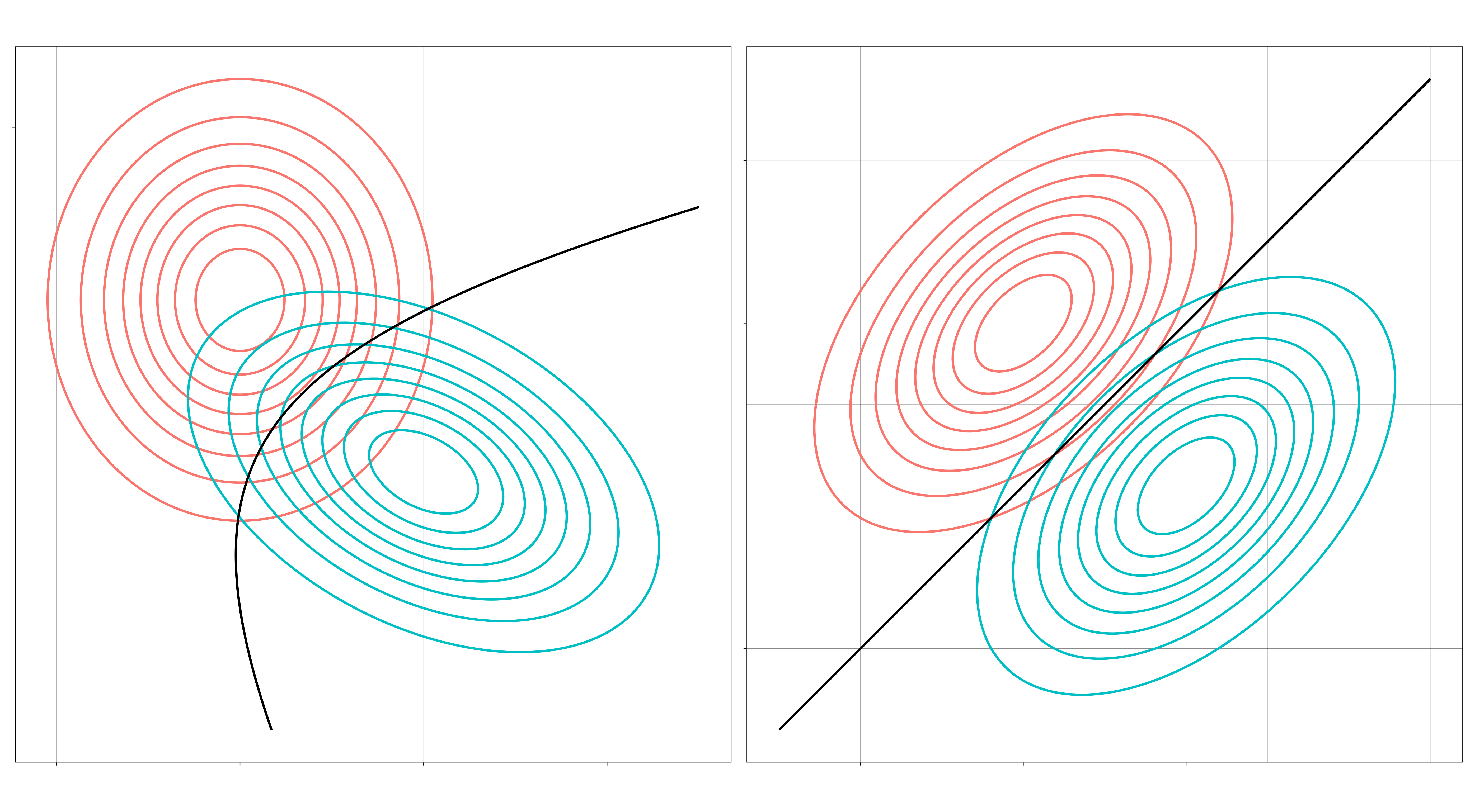
I. Are all the covariance matrices modeled separately, or is there one that they share? If separate, then the decision boundaries will be quadratic. If shared, then the decision boundaries will be linear. (Separate means \(\Sigma_c \neq \Sigma_d\) when \(c \neq d\). Shared means \(\Sigma_c = \Sigma\) for all \(c\).)

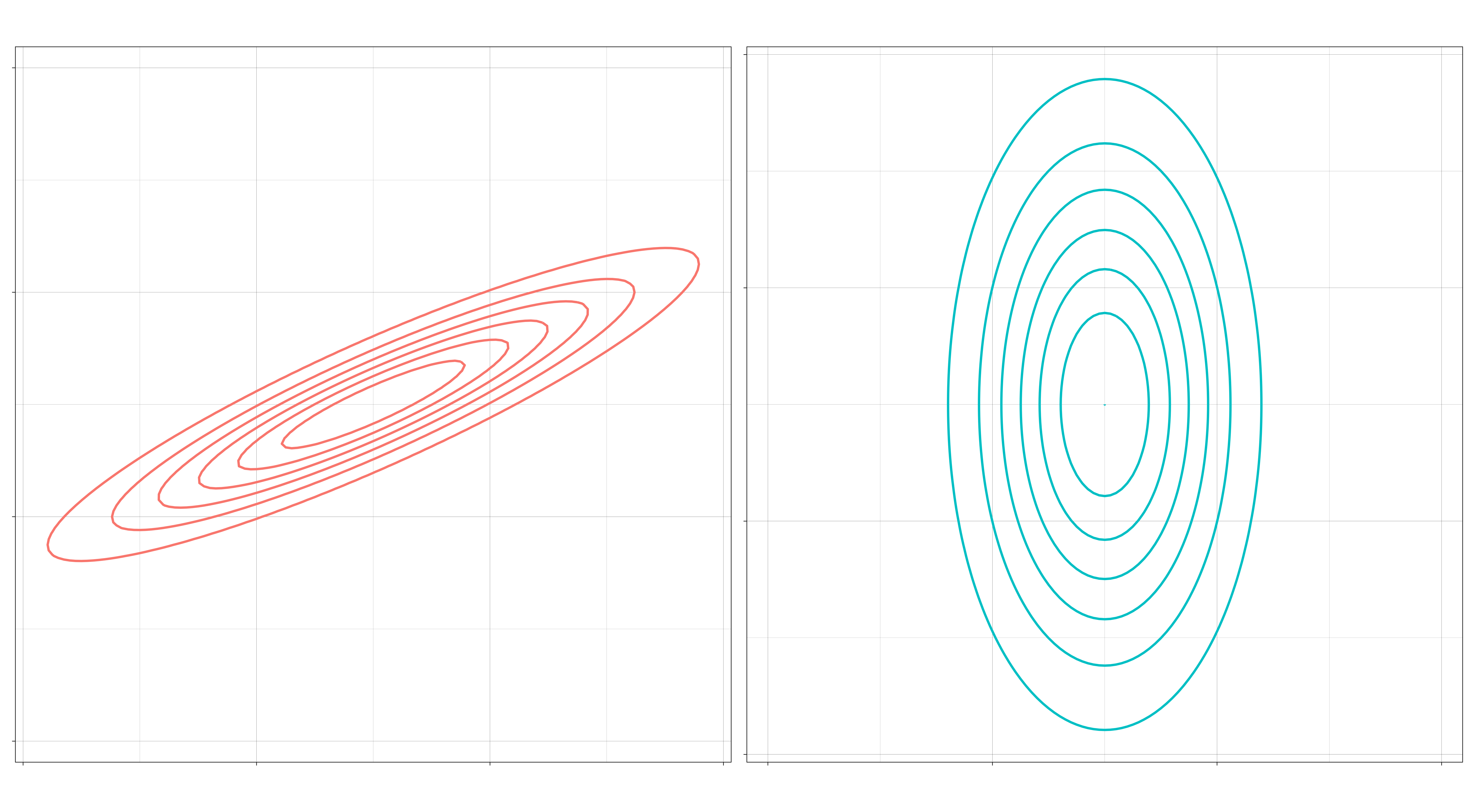
II. May the features within a class be correlated? If correlated, then the elliptical contours of the distribution will be at an angle. If independent, then they can only vary independently along each axis (up and down, left and right). (Independent means \(\Sigma_k\) is a diagonal matrix for all \(k\).)

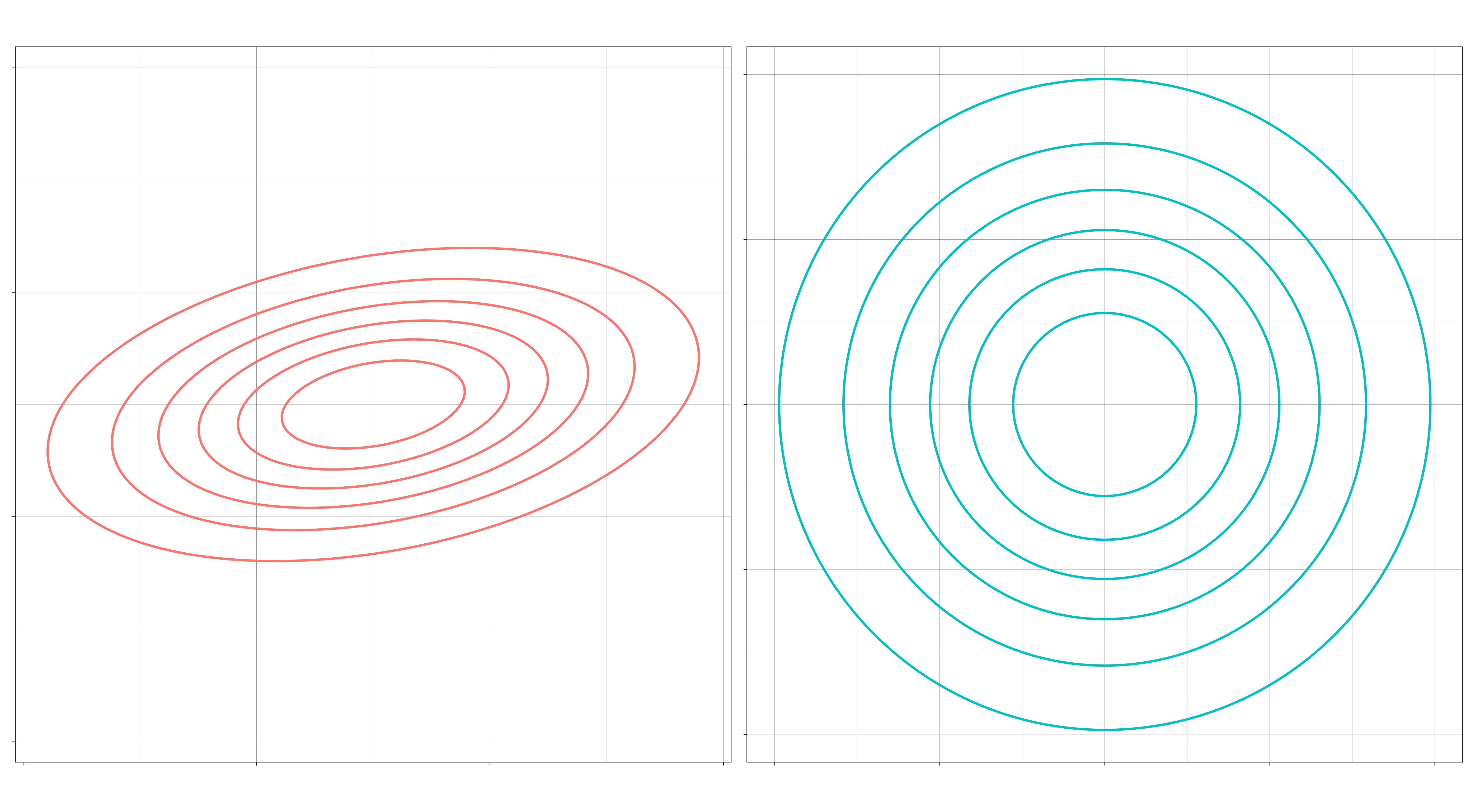
III. If the features within a class are uncorrelated, might they still differ by their standard deviations? If so, then the contours of the distribution can be elliptical. If not, then the contours will be spherical. (“No” means \(\Sigma_k = \sigma_k I\) for each \(k\), a multiple of the identity matrix.)

This gives us six different kinds of Gaussian disciminant analysis.

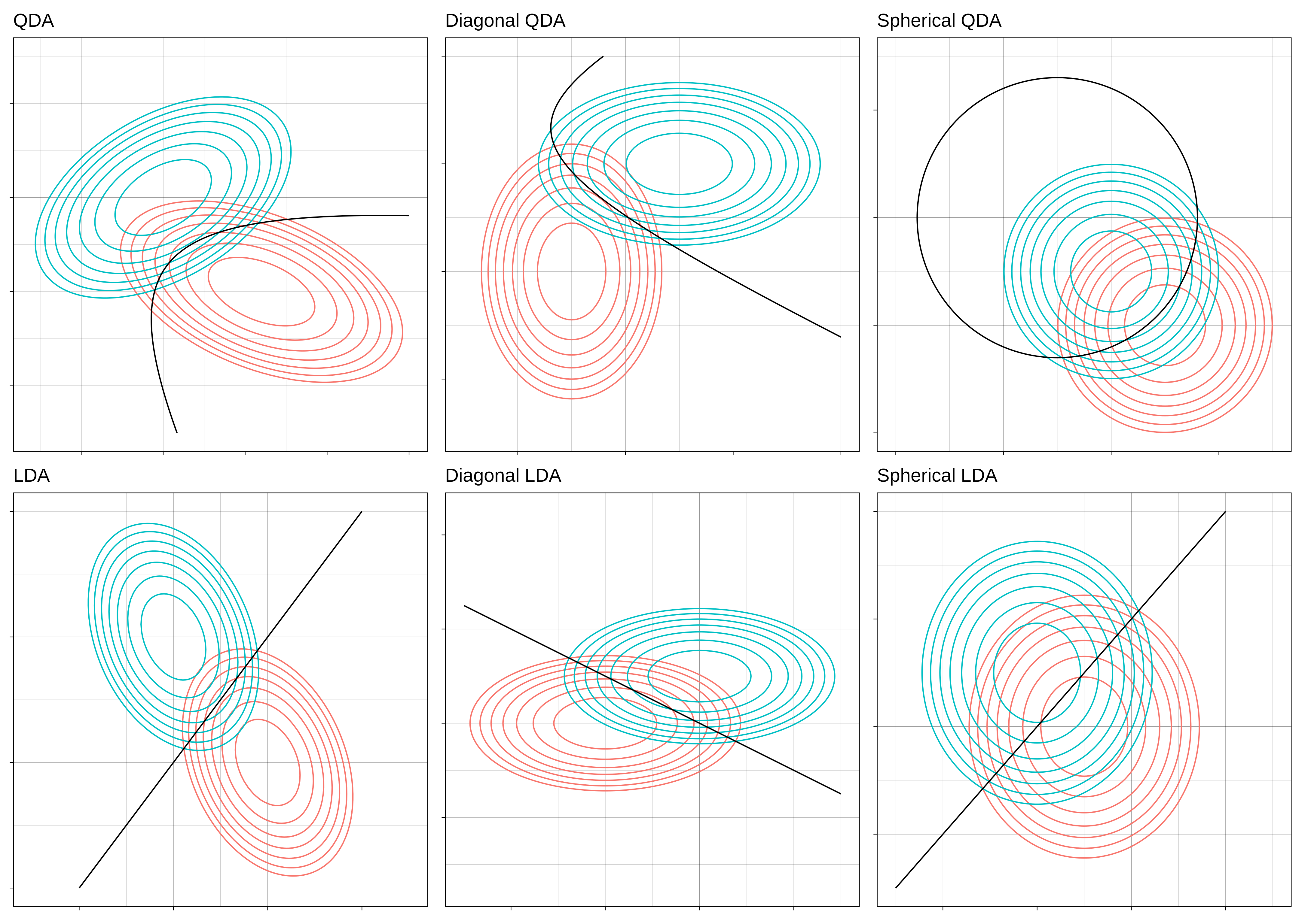
The more “no”s to these questions, the more restrictive the model is, and the more stable its decision boundary will be.

Whether this is good or bad depends on the data to which the model is applied. If there are a large number of observations relative to the number of features (a very long dataset), then the data can support a model with weaker assumptions. More flexible models require larger datasets in order to learn properties of the distributions that were not “built-in” by assumptions. The payoff is that there is less chance that the resulting model will differ a great deal from the true model.

But a model with the regularizing effect of strong assumptions might perform better when the number of observations is small relative to the number of features (a very wide dataset). Especially in high dimenions, the data may be so sparse that the classes are still well-separated by linear boundaries, even if the true boundaries are not linear. In very high-dimensional spaces (\(p > N\), there is not even enough data to obtain the MLE estimate, in which case some kind of regularization is necessary to even begin the problem.

So so that we know what kinds of assumptions we can make about \(\Sigma_k\), let’s take a look at how they affect the properties of the classifier.

Quadratic vs Linear

The most common distinction in discriminant classifiers is the distinction between those that have quadratic boundaries and those that have linear boundaries. As mentioned, the former go by quadratic discriminant analysis and the latter by linear discriminant analysis.

Recall the discriminant function for the general case:

\[ \delta_c(x) = -\frac{1}{2}(x - \mu_c)^\top \Sigma_c^{-1} (x - \mu_c) - \frac{1}{2}\log |\Sigma_c| + \log \pi_c \]

Notice that this is a quadratic function: \(x\) occurs twice in the first term. We obtain the decision boundary between two classes \(c\) and \(d\) by setting equal their discriminant functions \( \delta_c(x) - \delta_d(x) = 0 \). The set of solutions to this equation is the decision boundary. Whenever the covariance matrices \(\Sigma_c\) and \(\Sigma_d\) are distinct, this will be a quadric equation forming a quadric surface. In two dimensions, these surfaces are the conic sections: parabolas, hyperbolas, and ellipses.

Now let’s assume the covariance matrix \(\Sigma\) is the same for every class. After simplification of the equation \(\delta_c(x) - \delta_d(x) = 0\), there remains in this case only a single term depending on \(x\)

\[ x^\top \Sigma^{-1}(\mu_c - \mu_d) \]

which is linear in \(x\). This means the decision boundary is given by a linear equation, and the boundary is a hyperplane, which in two dimensions is a line.

Correlated vs Uncorrelated

The first question (quadratic vs. linear) concerned the relationship between the features of each class and thus determined the shape of the boundaries that separate them. The next two questions are about the classes individually. These questions concern the shape of the distributions themselves.

The second question asks whether we model the features within a class as being correlated or not. Recall the form of a covariance matrix for two variables,

\[\Sigma = \begin{bmatrix}\operatorname{Var}(X_1) & \operatorname{Cov}(X_1, X_2) \\ \operatorname{Cov}(X_2, X_1) & \operatorname{Var}(X_2)\end{bmatrix}\]

Whenever the RVs are uncorrelated, the covariance entries will equal 0, and the matrix becomes diagonal,

\[\Sigma = \begin{bmatrix}\operatorname{Var}(X_1) & 0 \\ 0 & \operatorname{Var}(X_2)\end{bmatrix}\]

In this case, each feature can only vary individually along its own axis. Thinking about the covariance matrix as a linear transformation, this means that the distribution’s elliptical contours are obtained through a scaling transform applied to circles. In other words, the contours can vary through stretching and shrinking along an axis, but not through a rotation.

The boundaries formed are quadratic because the two distributions have unequal covariances. If we kept the covariance matrices the same, all of the boundaries would remain linear.

When normally distributed variables are uncorrelated, they are also independent. This means that the diagonal models here are Naive Bayes classifiers.

Elliptical vs Spherical

The final question question concerns whether we put an additional constraint on diagonal covariance matricies, namely, whether we restrict the variances of the two features within a class to be equal. Calling this common variance \(\sigma^2\), such matrices look like

\[\Sigma = \begin{bmatrix} \sigma^2 & 0 \\ 0 & \sigma^2 \end{bmatrix} = \sigma^2 \begin{bmatrix} 1 & 0 \\ 0 & 1 \end{bmatrix} = \sigma^2 I\]

So, such matrices are simply scalar multiples of an identity matrix. The contours of the class-conditional distributions are spheres, and the decision boundaries themselves are also spherical.

Applied to standardized observations, a model of this sort would simply classify observations based upon their distance to the class means. In this way, Spherical LDA is equivalent to the nearest centroid classifier.

Model Mis-specification

The performance of a classifier will depend on how well its decision rule models the true data-generating distribution. The GDA family attempts to model the true distribution directly, and its performance will depend on how closely the true distribution resembles the chosen \(Normal(\mu_c, \Sigma_c)\).

What happens when the model diverges from the truth? Generally, the model will either not be flexible enough to fit the true decision boundary (inducing bias), or it will be overly flexible and will tend to overfit the data (inducing variance). In the first case, no amount of data will ever achieve the optimal error rate, while in the second case, the classifier does not use its data efficiently; in high dimensional domains, the amount of data needed to fit an under-specified model may be intractable.

To get a sense for these phenomena, let’s observe the behavior of a few of our GDA classifiers when we fit them on another distribution’s data model.

Example

In this example, the data was generated from a Diagonal QDA model. Show below are the LDA, Diagonal QDA, and QDA classifiers being fit to samples of increasing size.

What we should notice is that the LDA model never achieves a good fit to the optimal boundary because it is constrained in a way inconsistent with the true model. On the other hand, the QDA model does achieve a good fit, but it requires more data to do so than the Diagonal QDA model. (Incidentally, I think the odd shape of the Diagonal QDA model in the center is an artifact of the way the {sparsediscrim} package constructs its decision rule. Apparently, it does so through some kind of linear sum. In any case, it seems quite efficient.)