,
Published: January 9, 2020

Introduction

Over the next few posts, we will investigate decision boundaries. A decision boundary is a graphical representation of the solution to a classification problem. Decision boundaries can help us to understand what kind of solution might be appropriate for a problem. They can also help us to understand the how various machine learning classifiers arrive at a solution.

In this post, we will look at a problem’s optimal decision boundary, which we can find when we know exactly how our data was generated. The optimal decision boundary represents the “best” solution possible for that problem. Consequently, by looking at the complexity of this boundary and at how much error it produces, we can get an idea of the inherent difficulty of the problem.

Unless we have generated the data ourselves, we won’t usually be able to find the optimal boundary. Instead, we approximate it using a classifier. A good machine learning classifier tries to approximate the optimal boundary for a problem as closely as possible.

In future posts, we will look at the approximating boundary created by various classification algorithms. We will investigate the strategy the classifier uses to create this boundary and how this boundary evolves as the classifier is trained on more and more data. There are many classification algorithms available to a data scientist – regression, discriminant analysis, decision trees, neural networks, to name a few – and it is important to understand which algorithm is appropritate for the problem at hand. Decision boundaries can help us to do this.

Optimal Boundaries

A classification problem asks: given some observations of a thing, what is the best way to assign that thing to a class based on some of its features? For instance, we might want to predict whether a person will like a movie or not based on some data we have about them, the “features” of that person.

A solution to the classification problem is a rule that partitions the features and assigns each all the features of a partition to the same class. The “boundary” of this partitioning is the decision boundary of the rule.

It might be that two observations have exactly the same features, but are assigned to different classes. (Two things that look the same in the ways we’ve observed might differ in ways we haven’t observed.) In terms of probabilities this means both \[P(C = 0 \mid X) \gt 0\] and \[P(C = 1 \mid X) \gt 0\]. In other words, we might not be able with full certainty to classify an observation. We could however assign the observation to its most probable class. This gives us the decision rule \[ \hat{C} = \operatorname*{argmax}_c P(C = c \mid X) \]

The boundary that this rule produces is the optimal decision boundary. It is the MAP estimate of the class label, and it is the rule that minimizes classification error under the zero-one loss function. We will look at error and loss more in a future post.

We will consider binary classification problems, meaning, there will only be two possible classes, 0 or 1. For a binary classification problem, the optimal boundary occurs at those points where each class is equally probable: \[ P(C = 0 \mid X) = P(C = 1 \mid X) \]

Prepare R

We will use R to do our analysis. We’ll have a chance to try out gganimate and patchwork, a couple of newer packages that Thomas Lin Pedersen has been working on; they are really nice.

Here we’ll define some functions to produce plots of our examples. All of these assume a classification problem where our response is binary, \(C \in \{0, 1\}\), and is predicted by two continuous features, \((X, Y)\).

Briefly, they are

  1. gg_sample :: creates a layer for a sample of the features colored by class.
  2. gg_density :: creates a layer of contour plots for feature densities within each class.
  3. gg_optimal :: creates a layer showing an optimal decision boundary.
  4. gg_mix_label :: creates a layer labelling components in a mixture distribution.

library(magrittr)
library(tidyverse)
library(ggplot2)
library(gganimate)
library(patchwork)

theme_set(theme_linedraw() +
          theme(plot.title = element_text(size = 20),
                legend.position = "none",
                axis.text.x = element_blank(),
                axis.text.y = element_blank(),
                axis.title.x = element_blank(),
                axis.title.y = element_blank(),
                aspect.ratio = 1))

#' Make a sample layer
#'
#' @param data data.frame: a sample with continuous features `x` and `y`
#' grouped by factor `class`
#' @param classes (optional) a vector of which levels of `class` to
#' plot; default is to plot data from all classes
gg_sample <- function(data, classes = NULL, size = 3, alpha = 0.5, ...) {
    if (is.null(classes)) {
        subdata <- data
    } else {
        subdata <- filter(data, class %in% classes)
    }
    list(geom_point(data = subdata,
                    aes(x, y,
                        color = factor(class),
                        shape = factor(class)),
                    size = size,
                    alpha = alpha,
                    ...),
         scale_colour_discrete(drop = TRUE,
                               limits = levels(factor(data$class))))
}

#' Make a density layer
#'
#' @param data data.frame: a data grid of features `x` and `y` with contours `z`
#' @param data character: the name of the contour column 
gg_density <- function(data, z, size = 1, color = "black", alpha = 1, ...) {
    z <- ensym(z)
    geom_contour(data = data,
                 aes(x, y, z = !!z),
                 size = size,
                 color = color,
                 alpha = alpha,
                 ...)
}

#' Make an optimal boundary layer
#'
#' @param data data.frame: a data grid of features `x` and `y` with a column with
#' the `optimal` boundary contours
#' @param breaks numeric: which contour levels of `optimal` to plot
gg_optimal <- function(data, breaks = c(0), ...) {
    gg_density(data, z = optimal, breaks = breaks, ...)
}

#' Make a layer of component labels for a mixture distribution with two classes
#'
#' @param mus list(data.frame): the means for components of each class; every row
#' is a mean, each column is a coordinate
#' @param classes (optional) a vector of which levels of class to plot
gg_mix_label <- function(mus, classes = NULL, size = 10, ...) {
    ns <- map_int(mus, nrow)
    component <- do.call(c, map(ns, seq_len))
    class <- do.call(c, map2(0:(length(ns) - 1), ns, rep.int))
    mu_all <- do.call(rbind, mus)
    data <- cbind(mu_all, component, class) %>%
        set_colnames(c("x", "y", "component", "class")) %>%
        as_tibble()
    if (is.null(classes)) {
        subdata <- data
    } else {
        subdata <- filter(data, class %in% classes)
    }    
    list(shadowtext::geom_shadowtext(data = subdata,
                                     mapping = aes(x, y,
                                                   label = component,
                                                   color = factor(class)),
                                     size = size,
                                     ...),
         scale_colour_discrete(drop = TRUE,
                               limits = levels(factor(data$class))))
}

Decision Boundaries for Continuous Features

Decision boundaries are most easily visualized whenever we have continuous features, most especially when we have two continuous features, because then the decision boundary will exist in a plane.

With two continuous features, the feature space will form a plane, and a decision boundary in this feature space is a set of one or more curves that divide the plane into distinct regions. Inside of a region, all observations will be assigned to the same class.

As mentioned above, whenever we know exactly how our data was generated, we can produce the optimal decision boundary. Though this won’t usually be possible in practice, investigating the optimal boundaries produced from simulated data can still help us to understand their properties.

We will look at the optimal boundary for a binary classification problem on a with features on a couple of common distributions: a multivariate normal distribution and a mixture of normal distributions.

Normally Distributed Features

In a binary classification problem, whenever the features for each class jointly have a multivariate normal distribution, the optimal decision boundary is relatively simple. We will start our investigation here.

With two features, the feature space is a plane. It can be shown that the optimal decision boundary in this case will either be a line or a conic section (that is, an ellipse, a parabola, or a hyperbola). With higher dimesional feature spaces, the decision boundary will form a hyperplane or a quadric surface.

We will consider classification problems with two classes, \(C = {0, 1}\), and two features, \(X\) and \(Y\). Each class will be Bernoulli distributed and the features for each class will be distributed normally. Specifically,

Classes \( C \sim \operatorname{Bernoulli}(p) \)
Features for Class 0 \( (X, Y) \mid C = 0 \sim \operatorname{Normal}(\mu_0, \Sigma_0) \)
Features for Class 1 \( (X, Y) \mid C = 1 \sim \operatorname{Normal}(\mu_0, \Sigma_1) \)

Our goal is to produce two kinds of visualizations: one, of a sample from these distributions, and two, the contours of the class-conditional densities for each feature. We’ll use the mvnfast package to help us with computations on the joint MVN.

Samples

Let’s choose some values for our parameters. We’ll start with the case when the classes occur equally often. For our features, we’ll choose means so that there is some significant overlap between the two classes, and covariance matrices so that the distributions have a nice elliptical shape.

p <- 0.5
mu_0 <- c(0, 2)
sigma_0 <- matrix(c(1, 0.3, 0.3, 1), nrow = 2)
mu_1 <- c(2, 0)
sigma_1 <- matrix(c(1, -0.3, -0.3, 1), nrow = 2)

Now we’ll write a function to create a dataframe containing a sample of classified features from our distribution.

#' Generate normally distributed feature samples for a binary
#' classification problem
#'
#' @param n integer: the size of the sample
#' @param mean_0 vector: the mean vector of the first class
#' @param sigma_0 matrix: the 2x2 covariance matrix of the first class
#' @param mean_1 vector: the mean vector of the second class
#' @param sigma_1 matrix: the 2x2 covariance matrix of the second class
#' @param p_0 double: the prior probability of class 0
make_mvn_sample <- function(n, mu_0, sigma_0, mu_1, sigma_1, p_0) {
    n_0 <- rbinom(1, n, p_0)
    n_1 <- n - n_0
    sample_mvn <- as_tibble(
        rbind(mvnfast::rmvn(n_0,
                            mu = mu_0,
                            sigma = sigma_0),
              mvnfast::rmvn(n_1,
                            mu = mu_1,
                            sigma = sigma_1)))
    sample_mvn[1:n_0, 3] <- 0
    sample_mvn[(n_0 + 1):(n_0 + n_1), 3] <- 1
    sample_mvn <- sample_mvn[sample(nrow(sample_mvn)), ]
    colnames(sample_mvn) <- c("x", "y", "class")
    sample_mvn
}

Finally, we’ll create a sample of 4000 points and plot the result.

n <- 4000
set.seed(31415)
sample_mvn <- make_mvn_sample(n,
                              mu_0, sigma_0,
                              mu_1, sigma_1,
                              p)

ggplot() +
    gg_sample(sample_mvn) +
    coord_fixed()
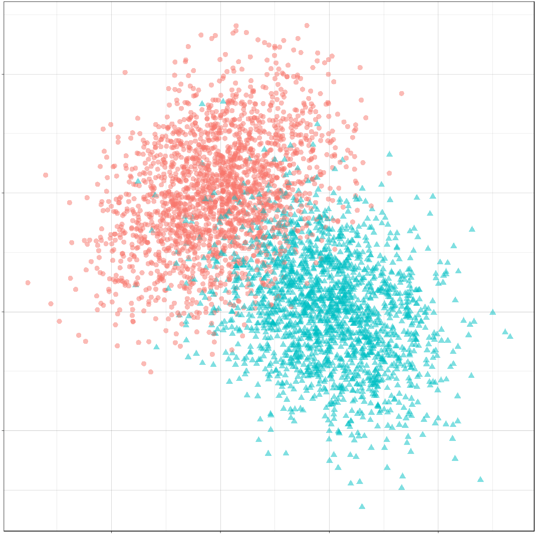
It should be apparent that because of the overlap in these distributions, any decision rule will necessarily misclassify some observations fairly often.

Classes on the Feature Space

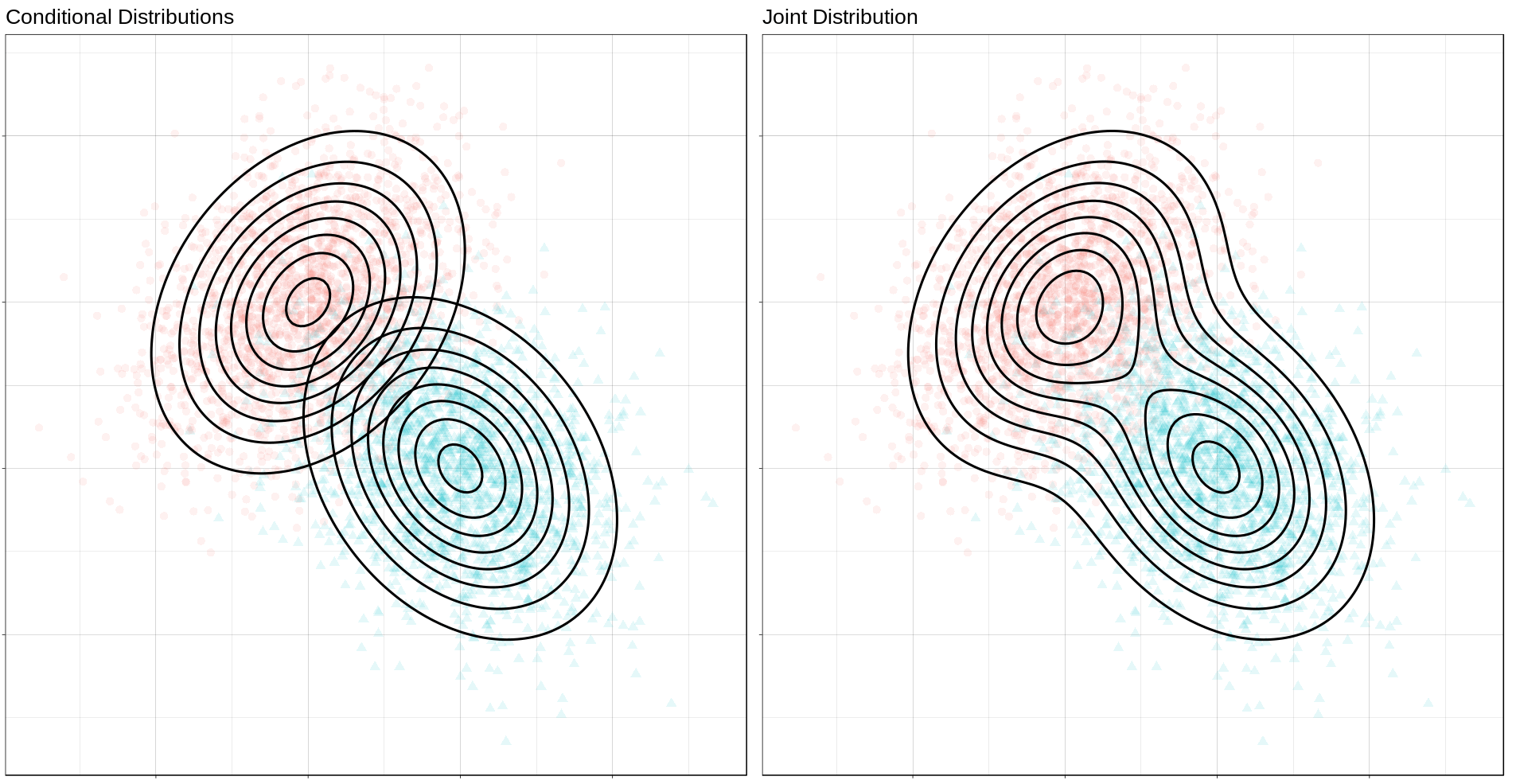
Next, we will produce some contour plots of our feature distributions. Let’s write a function to generate class probabilities at any observation \((x, y)\) in the feature space; we will model the optimal decision boundary as those points where the posterior probabilities of the two classes are equal, that is, where \[ P(X, Y \mid C = 0) P(C = 0) - P(X, Y \mid C = 1) P(C = 1) = 0 \]

#' Make an optimal prediction at a point from two class distributions
#'
#' @param x vector: input
#' @param p_0 double: prior probability of class 0
#' @param dfun_0 function(x): density of features of class 0
#' @param dfun_1 function(x): density of features of class 1
optimal_predict <- function(x, p_0, dfun_0, dfun_1) {
    ## Prior probability of class 1
    p_1 <- 1 - p_0
    ## Conditional probability of (x, y) given class 0
    p_x_0 <- dfun_0(x)
    ## Conditional probability of (x, y) given class 1
    p_x_1 <- dfun_1(x)
    ## Conditional probability of class 0 given (x, y)
    p_0_xy <- p_x_0 * p_0
    ## Conditional probability of class 1 given (x, y)
    p_1_xy <- p_x_1 * p_1
    optimal <- p_1_xy - p_0_xy
    class <- ifelse(optimal > 0, 1, 0)
    result <- c(p_0_xy, p_1_xy, optimal, class)
    names(result) <- c("p_0_xy", "p_1_xy", "optimal", "class")
    result
}

#' Construct a dataframe with posterior class probabilities and the
#' optimal decision boundary over a grid on the feature space
#' 
#' @param mean_0 vector: the mean vector of the first class
#' @param sigma_0 matrix: the 2x2 covariance matrix of the first class
#' @param mean_1 vector: the mean vector of the second class
#' @param sigma_1 matrix: the 2x2 covariance matrix of the second class
#' @param p_0 double: the prior probability of class 0
make_density_mvn <- function(mean_0, sigma_0, mean_1, sigma_1, p_0,
                             x_min, x_max, y_min, y_max, delta = 0.05) {
    x <- seq(x_min, x_max, delta)
    y <- seq(y_min, y_max, delta)
    density_mvn <- expand.grid(x, y)
    names(density_mvn) <- c("x", "y")
    dfun_0 <- function(x) mvnfast::dmvn(x, mu_0, sigma_0)
    dfun_1 <- function(x) mvnfast::dmvn(x, mu_1, sigma_1)
    optimal_mvn <- function(x, y) optimal_predict(c(x, y), p_0, dfun_0, dfun_1)
    density_mvn <-as.tibble(
        cbind(density_mvn,
              t(mapply(optimal_mvn,
                       density_mvn$x, density_mvn$y))))
    density_mvn
}

Now we can generate a grid of points and compute posterior class probabilities over that grid. By plotting these probabilities, we can get describe both the conditional feature distributions for each class as well as the joint feature distribution.

density_mvn <- make_density_mvn(mu_0, sigma_0, mu_1, sigma_1, p,
                                -3, 5, -3, 5)

(ggplot() +
 gg_sample(sample_mvn, alpha = 0.1) +
 gg_density(density_mvn, z = p_0_xy) +
 gg_density(density_mvn, z = p_1_xy) +
 ggtitle("Conditional Distributions")) +
(ggplot() +
 gg_sample(sample_mvn, alpha = 0.1) +
 geom_contour(data = density_mvn,
              aes(x = x, y = y, z = p_0_xy + p_1_xy),
              size = 1,
              color = "black") +
 ggtitle("Joint Distribution"))
The Optimal Decision Boundary

Now let’s add a plot for the optimal decision boundary for this problem.

(ggplot() +
 gg_density(density_mvn, z = p_0_xy,
            alpha = 0.25) +
 gg_density(density_mvn, z = p_1_xy,
            alpha = 0.25) +
 gg_optimal(density_mvn)) +
(ggplot() +
 gg_sample(sample_mvn, alpha = 0.25) +
 gg_optimal(density_mvn)) +
plot_annotation("The Optimal Decision Boundary")
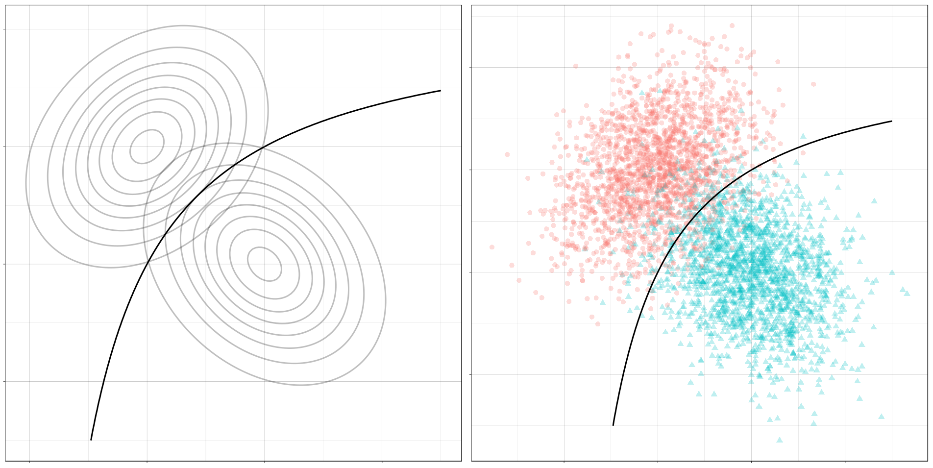
Notice how the boundary runs through the points where the contours of the two conditional distributions intersect. These points of intersection are where the classes have equal posterior probability.

Mixture of Normals

The features of each class might also be modeled as a mixture of normal distributions. This means that each observation in a class will come from one of several normal distributions; in our case, the distributions from a class will be joined by a common hyperparameter, their mean.

In description, at least, the problem is still relatively simple. The possible decision boundaries produced, however, can be quite complex. This is a much more difficult problem than the one we saw before.

For our examples, we will generate the data as follows:

Classes \( C \sim Bernoulli(p) \)
Mean of Means for Class 0 \( \nu_0 \sim Normal((0, 1), I) \)
Mean of Means for Class 1 \( \nu_0 \sim Normal((1, 0), I) \)
Means of Components for Class 0 \( \mu_{0, i=1, \ldots, n_0} \sim Normal(\nu_0, I) \)
Means of Components for Class 1 \( \mu_{1, i=1, \ldots, n_1} \sim Normal(\nu_1, I) \)
Features for Class 0 \( (X, Y) \mid C = 0 \sim w_{0, 1} Normal(\mu_{0, 1}, \Sigma_0) + \cdots + w_{0, l_0} Normal(\mu_{0, 0}, \Sigma_0) \)
Features for Class 1 \( (X, Y) \mid C = 1 \sim w_{1, 1} Normal(\mu_{1, 1}, \Sigma_1) + \cdots + w_{1, l_1} Normal(\mu_{1, l_1}, \Sigma_1) \)

where \(n_0\) is the number of components for class 0, \(w_{0, i}\) are the weights on each component, \(\Sigma_0 = \frac{1}{2 * l_0} I\), and \(I\) is the identity matrix; similarly for class 1.

This is a bit awful, but we are basically doing this:

For each class, define the distribution of the features \((X, Y)\) by

  1. Choosing the number of components to go in the mixture.
  2. Choosing a mean for each component by sampling from a normal distribution.

Then, to get a sample: Get an observation by

  1. Choosing a class, 0 or 1.
  2. Choosing a component from that class, a normal distribution.
  3. Sample the observation from that component.

Samples

The computations for the mixture of MVNs are fairly similar to the ones we did before. First let’s define a sampling function. This function just implements the above steps.

#' Generate normally distributed feature samples for a binary
#' classification problem
#'
#' @param n integer: the size of the sample
#' @param nu_0 numeric: the average mean of the components of the first feature
#' @param sigma_0 matrix: covariance of components of the first feature
#' @param n_0 integer: class frequency of first feature in the sample
#' @param w_0 numeric: vector of weights for components of the first feature
#' @param mean_1 numeric: the average mean of the components of the second feature
#' @param sigma_1 matrix: covariance of components of the second feature
#' @param n_1 integer: class frequency of second feature in the sample
#' @param w_1 numeric: vector of weights for components of the second feature
#' @param p_0 double: the prior probability of class 0
make_mix_sample <- function(n,
                            nu_0, tau_0, n_0, sigma_0, w_0,
                            nu_1, tau_1, n_1, sigma_1, w_1,
                            p_0) {
    ## Number of Components for Each Class
    l_0 <- length(w_0)
    l_1 <- length(w_1)
    ## Sample the Component Means
    mu_0 <- mvnfast::rmvn(n = l_0,
                          mu = nu_0, sigma = tau_0)
    mu_1 <- mvnfast::rmvn(n = l_1,
                          mu = nu_1, sigma = tau_1)
    ## Class Frequency in the Sample
    n_0 <- rbinom(1, n, p_0)
    n_1 <- n - n_0
    ## Sample the Features
    f_0 <- mvnfast::rmixn(n = n_0,
                          mu = mu_0, sigma = sigma_0, w = w_0,
                          retInd = TRUE)
    c_0 <- attr(f_0, "index")
    f_1 <- mvnfast::rmixn(n = n_1,
                          mu = mu_1, sigma = sigma_1, w = w_1,
                          retInd = TRUE)
    c_1 <- attr(f_1, "index")
    sample_mix <- as.data.frame(rbind(f_0, f_1))
    sample_mix[, 3] <- c(c_0, c_1)
    ## Define Classes
    sample_mix[1:n_0, 4] <- 0
    sample_mix[(n_0 + 1):(n_0 + n_1), 4] <- 1
    sample_mix <- sample_mix[sample(nrow(sample_mix)), ]
    names(sample_mix) <- c("x", "y", "component", "class")
    ## Store Component Means
    attr(sample_mix, "mu_0") <- mu_0
    attr(sample_mix, "mu_1") <- mu_1
    sample_mix
}

Now we’ll define the parameters, construct a sample, and look at the result.


## Bernoulli parameter for class distribution
p = 0.5
## Mean of component means
nu_0 = c(0, 1)
nu_1 = c(1, 0)
## Covariance for component means
tau_0 = matrix(c(1, 0, 0, 1), nrow = 2)
tau_1 = matrix(c(1, 0, 0, 1), nrow = 2)
## Number of components for each class
n_0 <- 10
n_1 <- 10
## Covariance for each class
sigma_0 <- replicate(n_0, matrix(c(1, 0, 0, 1), 2) / n_0 * 2,
                     simplify = FALSE)
sigma_1 <- replicate(n_1, matrix(c(1, 0, 0, 1), 2) / n_1 * 2,
                     simplify = FALSE)
## Weights of mixture components
w_0 <- rep(1 / n_0, n_0)
w_1 <- rep(1 / n_1, n_1)

## Sample size
n <- 4000
set.seed(31)
sample_mix <- make_mix_sample(n,
                              nu_0, tau_0, n_0, sigma_0, w_0,
                              nu_1, tau_1, n_1, sigma_1, w_1,
                              p)
## Retrieve the generated component means
mu_0 <- attr(sample_mix, "mu_0")
mu_1 <- attr(sample_mix, "mu_1")

ggplot() +
    gg_sample(sample_mix) +
    ggtitle("Sample of Mixture Distribution")

ggplot() +
    gg_sample(sample_mix) +
    gg_mix_label(list(mu_0, mu_1)) +
    facet_wrap(vars(class)) +
    ggtitle("Feature Components")
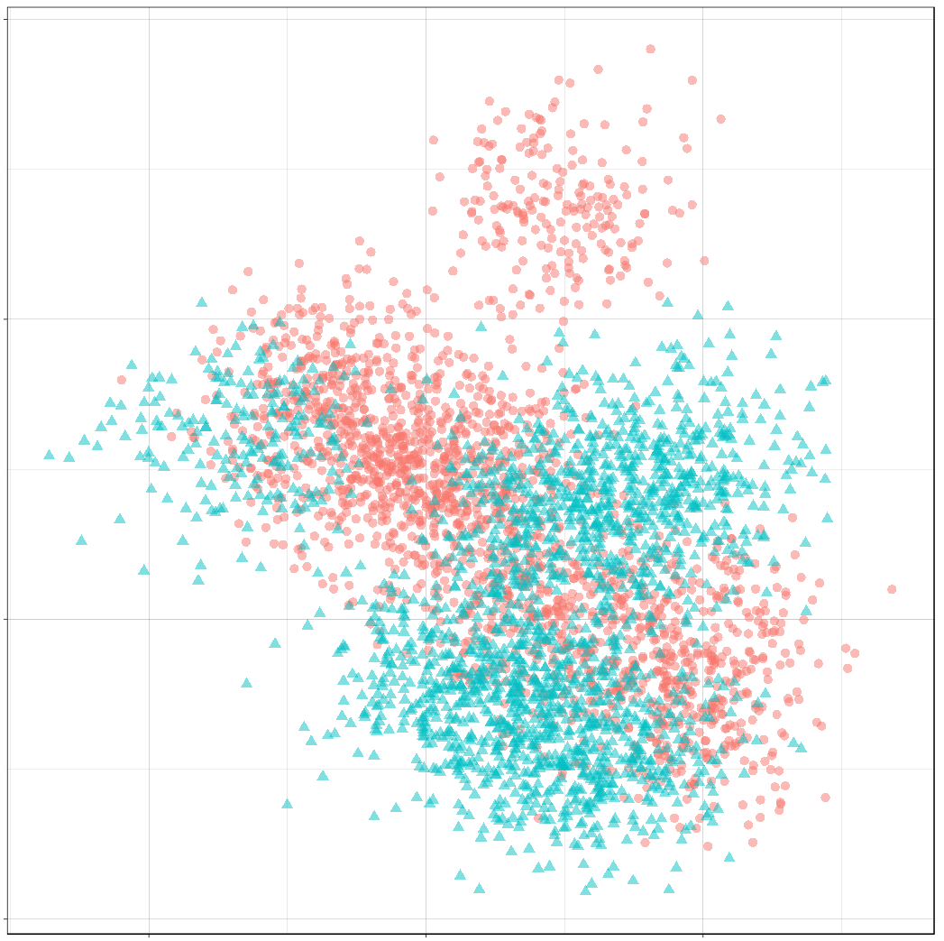
We’ve labelled the component means for each class. (There are 10 components for class 0, and 10 components for class 1.) You can see that around each of these labels is a sample from a normal distribution.

Classes on the Feature Space

Now we’ll compute class probabilities on the feature space.

First define a generating function.

#' Construct a dataframe with posterior class probabilities and the
#' optimal decision boundary over a grid on the feature space
#' 
#' @param mean_0 numeric: the average mean of the components of the first feature
#' @param sigma_0 matrix: covariance of components of the first feature
#' @param w_0 numeric: vector of weights for components of the first feature
#' @param mean_1 numeric: the average mean of the components of the second feature
#' @param sigma_1 matrix: covariance of components of the second feature
#' @param w_1 numeric: vector of weights for components of the second feature
#' @param p_0 double: the prior probability of class 0
make_density_mix <- function(mean_0, sigma_0, w_0,
                             mean_1, sigma_1, w_1, p_0,
                             x_min, x_max, y_min, y_max, delta = 0.05) {
    x <- seq(x_min, x_max, delta)
    y <- seq(y_min, y_max, delta)
    density_mix <- expand.grid(x, y)
    names(density_mix) <- c("x", "y")
    dfun_0 <- function(x) mvnfast::dmixn(matrix(x, nrow = 1),
                                         mu = mean_0,
                                         sigma = sigma_0,
                                         w = w_0)
    dfun_1 <- function(x) mvnfast::dmixn(matrix(x, nrow = 1),
                                         mu = mean_1,
                                         sigma = sigma_1,
                                         w = w_1)
    optimal_mix <- function(x, y) optimal_predict(c(x, y), p_0, dfun_0, dfun_1)
    density_mix <-as.tibble(
        cbind(density_mix,
              t(mapply(optimal_mix,
                       density_mix$x, density_mix$y))))
    density_mix
}

And now compute the grid and plot.

density_mix <- make_density_mix(mu_0, sigma_0, w_0, mu_1, sigma_1, w_1, p,
                                -3, 5, -3, 5)

(ggplot() +
 gg_sample(sample_mix, classes = 0,
           alpha = 0.1) +
 gg_density(density_mix, z = p_0_xy) +
 gg_mix_label(list(mu_0, mu_1), classes = 0) +
 ggtitle("Density of Class 0")) +
(ggplot() +
 gg_sample(sample_mix, classes = 1,
           alpha = 0.1) +
 gg_density(density_mix, z = p_1_xy) +
 gg_mix_label(list(mu_0, mu_1), classes = 1) +
 ggtitle("Density of Class 1")) +
(ggplot() +
 gg_sample(sample_mix,
           alpha = 0.1) +
 geom_contour(data = density_mix,
              aes(x = x, y = y, z = p_0_xy + p_1_xy),
              color = "black",
              size = 1) +
 ggtitle("Joint Density"))
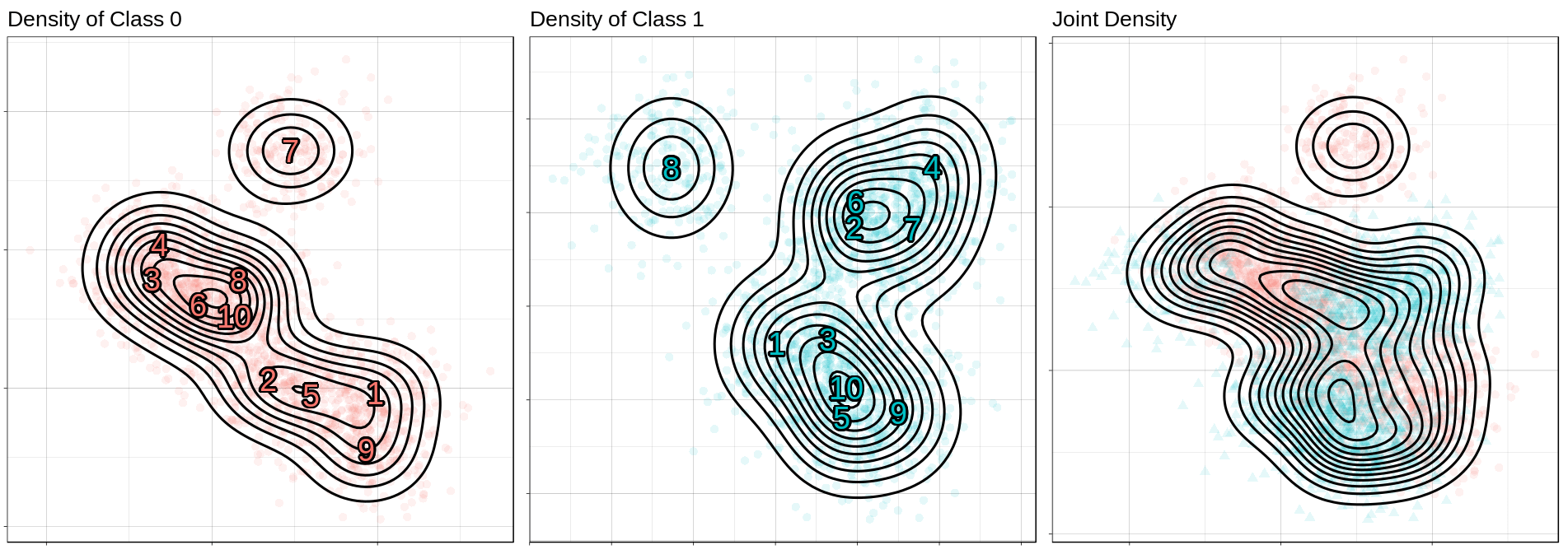
The Optimal Decision Boundary

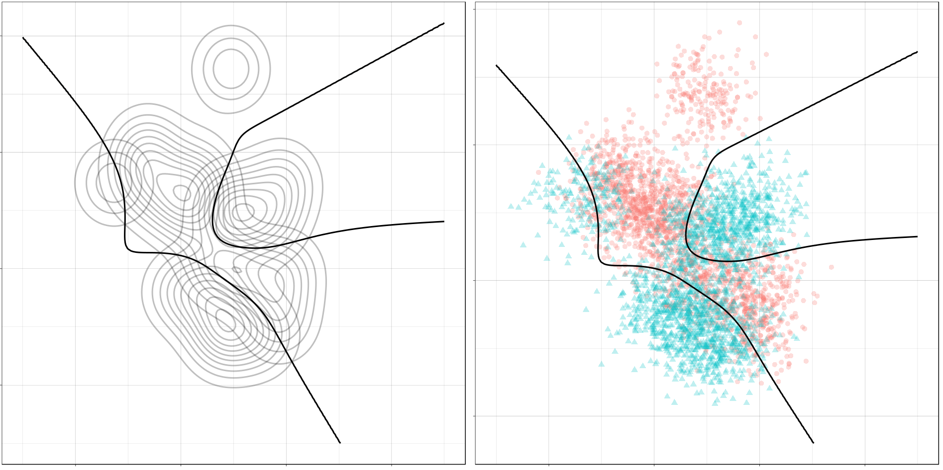
And here is the optimal decision boundary for this problem. Notice how again the boundary runs through points of intersection in the two conditional distributions, and how it separates the classes of observations in the sample.

(ggplot() +
 gg_density(density_mix, z = p_0_xy,
            alpha = 0.25) +
 gg_density(density_mix, z = p_1_xy,
            alpha = 0.25) +
 gg_optimal(density_mix)) +
(ggplot() +
 gg_sample(sample_mix, alpha = 0.25) +
 gg_optimal(density_mix))
Class Imbalance

So far, we’ve only seen the case where the two classes occur about equally often. If one class has a lower probability of occuring (say class 1), then the optimal decision boundary must move toward the class 1 distribution in order to equalize the probabilities on either side. This should help illustrate why it’s important to consider class imbalance whenever you’re working on a classification problem. A large imbalance can change your decisions drastically.

To see this change, we will use the gganimate package to produce an animation showing how the optimal boundary changes as the Bernoulli parameter (the frequency of class 0) changes from 0.1 to 0.9.

Normally Distributed Features

## Evaluate mu_0, sigma_0, etc. again, if needed.

density_p0 <-
    map_dfr(seq(0.1, 0.9, 0.005),
            function(p_0)
                make_density_mvn(mu_0, sigma_0, mu_1, sigma_1,
                                 p_0, -3, 5, -3, 5) %>%
                mutate(p_0 = p_0))

anim <- ggplot() +
    geom_contour(data = density_p0,
                 aes(x = x, y = y, z = p_0_xy + p_1_xy),
                 color = "black",
                 size = 1,
                 alpha = 0.25) +
    gg_optimal(density_p0) +
    transition_manual(p_0) +
    ggtitle("Proportion of Class 0: {current_frame}")

anim <- animate(anim, renderer = gifski_renderer(),
                width = 800, height = 800)

anim

Mixture of Normals

density_mix_p0 <-
    map_dfr(seq(0.1, 0.9, 0.005),
            function(p_0)
                make_density_mix(mu_0, sigma_0, w_0, mu_1, sigma_1, w_1,
                                 p_0, -3, 5, -3, 5) %>%
                mutate(p_0 = p_0))
anim <- ggplot() +
    geom_contour(data = density_mix_p0,
                 aes(x = x, y = y, z = p_0_xy + p_1_xy),
                 color = "black",
                 size = 1,
                 alpha = 0.25) +
    gg_optimal(density_mix_p0) +
    transition_manual(p_0) +
    ggtitle("Proportion of Class 0: {current_frame}")

anim <- animate(anim, renderer = gifski_renderer(),
                width = 800, height = 800)

anim

Conclusion

In this post, we reviewed decision boundaries, a way of visualizing classification rules. In particular, we looked at optimal decision boundaries, which represent the best solution possible to a problem given certain costs for misclassification. The rule we used in this post was the MAP estimate, which minimizes zero-one loss, where all misclassifications are equally likely.

In future posts, we’ll look other kinds of loss functions and how that can affect the decision rule, and also at the boundaries produced by a number of statistical learning models.

Hope you enjoyed it!
Introduction

The inverse of a matrix \(A\) is another matrix \(A^{-1}\) that has this property:

\[\begin{align*} A A^{-1} &= I \\ A^{-1} A &= I \end{align*} \]

where \(I\) is the identity matrix. This is a nice property for a matrix to have, because then we can work with it in equations just like we might with ordinary numbers. For instance, to solve some linear system of equations \[ A x = b \] we can just multiply the inverse of \(A\) to both sides \[ x = A^{-1} b \] and then we have some unique solution vector \(x\). Again, this is just like we would do if we were trying to solve a real-number equation like \(a x = b\).

Now, a matrix has an inverse whenever it is square and its rows are linearly independent. But not every system of equations we might care about will give us a matrix that satisfies these properties. The coefficient matrix \(A\) would fail to be invertible if the system did not have the same number of equations as unknowns (\(A\) is not square), or if the system had dependent equations (\(A\) has dependent rows).

Generalized inverses are meant to solve this problem. They are meant to solve equations like \(A x = b\) in the “best way possible” when \(A^{-1}\) fails to exist. There are many kinds of generalized inverses, each with its own “best way.” (They can be used to solve ridge regression problems, for instance.)

The most common is the Moore-Penrose inverse, or sometimes just the pseudoinverse. It solves the least-squares problem for linear systems, and therefore will give us a solution \(\hat{x}\) so that \(A \hat{x}\) is as close as possible in ordinary Euclidean distance to the vector \(b\).

The notation for the Moore-Penrose inverse is \(A^+\) instead of \(A^{-1}\). If \(A\) is invertible, then in fact \(A^+ = A^{-1}\), and in that case the solution to the least-squares problem is the same as the ordinary solution (\(A^+ b = A^{-1} b\)). So, the MP-inverse is strictly more general than the ordinary inverse: we can always use it and it will always give us the same solution as the ordinary inverse whenever the ordinary inverse exists.

We will look at how we can construct the Moore-Penrose inverse using the SVD. This turns out to be an easy extension to constructing the ordinary matrix inverse with the SVD. We will then see how solving a least-squares problem is just as easy as solving an ordinary equation.

Example - System with an Invertible Matrix

First let’s recall how to solve a system whose coefficient matrix is invertible. In this case, we have the same number of equations as unknowns and the equations are all independent. Then \(A^{-1}\) exists and we can find a unique solution for \(x\) by multiplying \(A^{-1}\) on both sides.

For instance, say we have

\[ \left\{\begin{align*} x_1 - \frac{1}{2}x_2 &= 1 \\ -\frac{1}{2} x_1 + x_2 &= -1 \end{align*}\right. \]

Then

\[ \begin{array}{c c} A = \begin{bmatrix} 1 & -1/2 \\ -1/2 & 1 \end{bmatrix}, &A^{-1} = \begin{bmatrix} 4/3 & 2/3 \\ 2/3 & 4/3 \end{bmatrix} \end{array} \]

and

\[x = A^{-1}b = \begin{bmatrix} 4/3 & 2/3 \\ 2/3 & 4/3 \end{bmatrix} \begin{bmatrix} 1 \\ -1 \end{bmatrix} = \begin{bmatrix} 2/3 \\ -2/3 \end{bmatrix} \]

So \(x_1 = \frac{2}{3}\) and \(x_2 = -\frac{2}{3}\).

Constructing Inverses with the SVD

The singular value decomposition (SVD) gives us an intuitive way constructing an inverse matrix. We will be able to see how the geometric transforms of \(A^{-1}\) undo the transforms of \(A\).

The SVD says that for any matrix \(A\),

\[ A = U \Sigma V^* \]

where \(U\) and \(V\) are orthogonal matricies and \(\Sigma\) is a diagonal matrix.

Now, if \(A\) is invertible, we can use its SVD to find \(A^{-1}\) like so:

\[ A^{-1} = V \Sigma^{-1} U^* \]

If we have the SVD of \(A\), we can construct its inverse by swapping the orthogonal matrices \(U\) and \(V\) and finding the inverse of \(\Sigma\). Since \(\Sigma\) is diagonal, we can do this by just taking reciprocals of its diagonal entries.

Example

Let’s look at our earlier matrix again:

\[ A = \begin{bmatrix} 1 & -1/2 \\ -1/2 & 1 \end{bmatrix} \]

It has SVD

\[ A = U \Sigma V^* = \begin{bmatrix} \sqrt{2}/2 & -\sqrt{2}/2 \\ \sqrt{2}/2 & \sqrt{2}/2 \end{bmatrix} \begin{bmatrix} 3/2 & 0 \\ 0 & 1/2 \end{bmatrix} \begin{bmatrix} \sqrt{2}/2 & \sqrt{2}/2 \\ -\sqrt{2}/2 & \sqrt{2}/2 \end{bmatrix} \]

And so,

\[ A^{-1} = V \Sigma^{-1} U^* = \begin{bmatrix} \sqrt{2}/2 & -\sqrt{2}/2 \\ \sqrt{2}/2 & \sqrt{2}/2 \end{bmatrix} \begin{bmatrix} 2/3 & 0 \\ 0 & 2 \end{bmatrix} \begin{bmatrix} \sqrt{2}/2 & \sqrt{2}/2 \\ -\sqrt{2}/2 & \sqrt{2}/2 \end{bmatrix} \]

and after multiplying everything out, we get

\[ A^{-1} = \begin{bmatrix} 4/3 & 2/3 \\ 2/3 & 4/3 \end{bmatrix} \]

just like we had before.

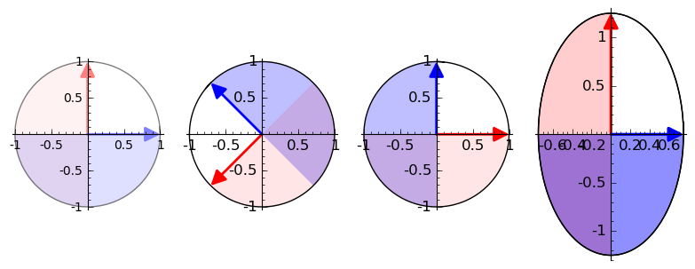
In an earlier post, we saw how we could use the SVD to visualize a matrix as a sequence of geometric transformations. Here is the matrix \(A\) followed by \(A^{-1}\), acting on the unit circle:

The inverse matrix \(A^{-1}\) reverses exactly the action of \(A\). The matrix \(A\) will map any circle to a unique ellipse, with no overlap. So, \(A^{-1}\) can map ellipses back to those same circles without any ambiguity. We don’t “lose information” by applying \(A\).

Constructing MP-Inverses with the SVD

We can in fact do basically the same thing for any matrix, not just the invertible ones. The SVD always exists, so for some matrix \(A\), first write

\[ A = U \Sigma V^* \]

And then find the MP-inverse by

\[ A^+ = V \Sigma^+ U^* \]

Now, the matrix \(A\) might not be invertible. If it is not square, then, to find \(\Sigma^+\), we need to take the transpose of \(\Sigma\) to make sure all the dimensions are conformable in the multiplication. It \(A\) is singular (dependent rows), then \(\Sigma\) will have 0’s on its diagaonal, so we need to make sure only take reciprocals of the non-zero entries.

Summarizing, to find the Moore-Penrose inverse of a matrix \(A\):

  1. Find the Singular Value Decomposition: \(A = U \Sigma V^*\) (using R or Python, if you like).
  2. Find \(\Sigma^+\) by transposing \(\Sigma\) and taking the reciprocal of all its non-zero diagonal entries.
  3. Compute \(A^+ = V \Sigma^+ U^*\)

Example - An Inconsistent System

Let’s find the MP-inverse of a singular matrix. Let’s take

\[A = \begin{bmatrix} 1 & 1 \\ 1 & 1 \end{bmatrix} \]

Because the rows of this matrix are linearly dependent, \(A^{-1}\) does not exist. But we can still find the more general MP-inverse by following the procedure above.

So, first we find the SVD of \(A\):

\[ A = U \Sigma V^* = \begin{bmatrix} \sqrt{2}/2 & -\sqrt{2}/2 \\ \sqrt{2}/2 & \sqrt{2}/2 \end{bmatrix} \begin{bmatrix} 2 & 0 \\ 0 & 0 \end{bmatrix} \begin{bmatrix} \sqrt{2}/2 & \sqrt{2}/2 \\ -\sqrt{2}/2 & \sqrt{2}/2 \end{bmatrix} \]

Then we apply the procedure above to find \(A^+\):

\[ A^+ = V \Sigma^+ U^* = \begin{bmatrix} \sqrt{2}/2 & -\sqrt{2}/2 \\ \sqrt{2}/2 & \sqrt{2}/2 \end{bmatrix} \begin{bmatrix} 1/2 & 0 \\ 0 & 0 \end{bmatrix} \begin{bmatrix} \sqrt{2}/2 & \sqrt{2}/2 \\ -\sqrt{2}/2 & \sqrt{2}/2 \end{bmatrix} \]

And now we multiply everything out to get:

\[ A^+ = \begin{bmatrix} 1/4 & 1/4 \\ 1/4 & 1/4 \end{bmatrix} \]

This is the Moore-Penrose inverse of \(A\).

Like we did for the invertible matrix before, let’s get an idea of what \(A\) and \(A^+\) are doing geometrically. Here they are acting on the unit circle:

Notice how \(A\) now collapses the circle onto a one-dimensional space. This is a consequence of it having dependent columns. For matricies with dependent columns, its image will be of lesser dimension than the space it’s mapping into. Another way of saying this is that it has a non-trivial null space. It “zeroes out” some of the dimensions in its domain during the transformation.

What if \(A\) were the coefficient matrix of a system of equations? We might have:

\[ \left\{ \begin{align*} x_1 + x_2 &= b_1 \\ x_1 + x_2 &= b_2 \end{align*} \right. \]

for some \(b_1\) and \(b_2\).

Now, unless \(b_1\) and \(b_2\) are equal, this system won’t have an exact solution for \(x_1\) and \(x_2\). It will be inconsistent. But, with \(A^+\), we can still find values for \(x_1\) and \(x_2\) that minimize the distance between \(A x\) and \(b\). More specifically, let \(\hat{x} = A^{+}b\). Then \(\hat{x}\) will minimize \(|| b - A x ||^2 \), the squared error, and \( \hat{b} = A \hat{x} = A A^{+} x \) is the closest we can come to \(b\). (The vector \(b - A \hat{x}\) is sometimes called the residual vector.)

We have

\[ \hat{x} = A^{+} b = \begin{bmatrix} 1/4 (b_1 + b_2) \\ 1/4 (b_1 + b_2) \end{bmatrix} \]

so \(x_1 = \frac{1}{4} (b_1 + b_2)\) and \(x_2 = \frac{1}{4} (b_1 + b_2)\). And the closest we can get to \(b\) is

\[ \hat{b} = A \hat{x} = \begin{bmatrix} 1/2 (b_1 + b_2) \\ 1/2 (b_1 + b_2) \end{bmatrix} \]

In other words, if we have to make \(x_1 + x_2\) as close as possible to two different values \(b_1\) and \(b_2\), the best we can do is to choose \(x_1\) and \(x_2\) so as to get the average of \(b_1\) and \(b_2\).

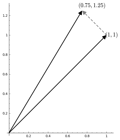
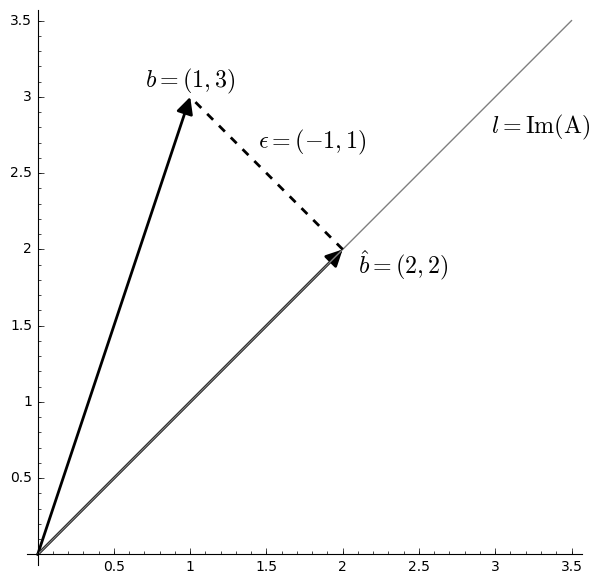
The vector \(b = (1, 3)\) and its orthogonal projection \(\hat{b} = (2, 2)\).

Or we could think about this problem geometrically. In order for there to be a solution to \(A x = b\), the vector \(b\) has to reside in the image of \(A\). The image of \(A\) is the span of its columns, which is all vectors like \(c(1, 1)\) for a scalar \(c\). This is just the line through the origin in the picture above. But \(b = (b_1, b_2)\) is not on that line if \(b_1 \neq b_2\), and so instead we minimize the distance between the two with its orthogonal projection \(\hat b\). The error or residual is the difference \(\epsilon = b - \hat{b}\).

, , ,
Published: November 15, 2019

Introduction

What are eigenvalues? What are singular values? They both describe the behavior of a matrix on a certain set of vectors. The difference is this: The eigenvectors of a matrix describe the directions of its invariant action. The singular vectors of a matrix describe the directions of its maximum action. And the corresponding eigen- and singular values describe the magnitude of that action.

They are defined this way. A scalar \(\lambda\) is an eigenvalue of a linear transformation \(A\) if there is a vector \(v\) such that \(A v = \lambda v\), and \(v\) is called an eigenvector of \(\lambda\). A scalar \(\sigma\) is a singular value of \(A\) if there are (unit) vectors \(u\) and \(v\) such that \(A v = \sigma u\) and \(A^* u = \sigma v\), where \(A^*\) is the conjugate transpose of \(A\); the vectors \(u\) and \(v\) are singular vectors. The vector \(u\) is called a left singular vector and \(v\) a right singular vector.

Eigenvalues and Eigenvectors

That eigenvectors give the directions of invariant action is obvious from the definition. The definition says that when \(A\) acts on an eigenvector, it just multiplies it by a constant, the corresponding eigenvalue. In other words, when a linear transformation acts on one of its eigenvectors, it shrinks the vector or stretches it and reverses its direction if \(\lambda\) is negative, but never changes the direction otherwise. The action is invariant.

Take this matrix, for instance:

\[ A = \begin{bmatrix} 0 & 2 \\ 2 & 0 \end{bmatrix} \]

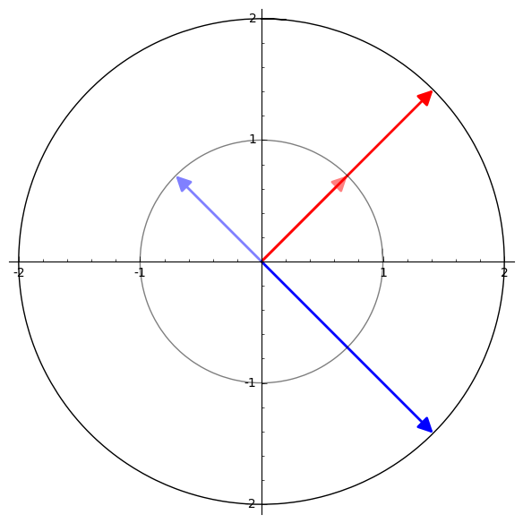
We can see how the transformation just stretches the red vector by a factor of 2, while the blue vector it stretches but also reflects over the origin.

And this matrix:

\[ A = \begin{bmatrix} 1 & \frac{1}{3} \\ \frac{4}{3} & 1 \end{bmatrix} \]

It stretches the red vector and shrinks the blue vector, but reverses neither.

The point is that in every case, when a matrix acts on one of its eigenvectors, the action is always in a parallel direction.

Singular Values and Singular Vectors

This invariant direction does not necessarily give the transformation’s direction of greatest effect, however. You can see that in the previous example. But say \(\sigma_1\) is the largest singular value of \(A\) with right singular vector \(v\). Then \(v\) is a solution to

\[ \operatorname*{argmax}_{x, ||x||=1} ||A x|| \]

In other words, \( ||A v|| = \sigma_1 \) is at least as big as \( ||A x|| \) for any other unit vector \(x\). It’s not necessarily the case that \(A v\) is parallel to \(v\), though.

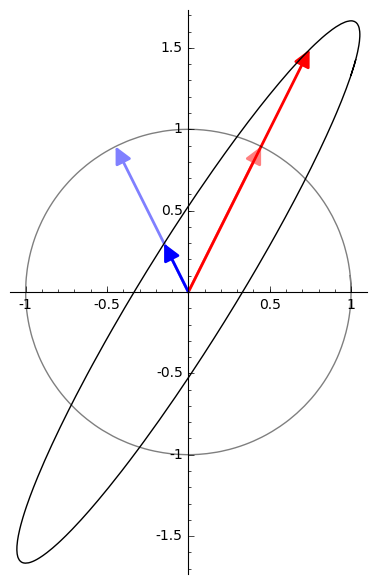
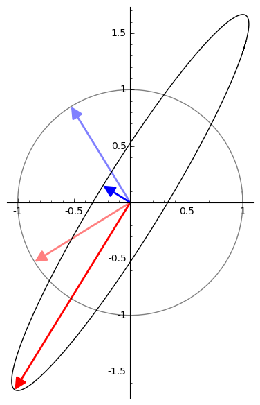
Compare the eigenvectors of the matrix in the last example to its singular vectors:

The directions of maximum effect will be exactly the semi-axes of the ellipse, the ellipse which is the image of the unit circle under \(A\).

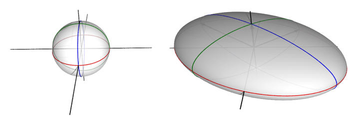
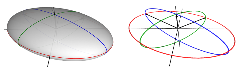
Let’s extend this idea to 3-dimensional space to get a better idea of what’s going on. Consider this transformation:

\[A = \begin{bmatrix} \frac{3}{2} \, \sqrt{2} & -\sqrt{2} & 0 \\ \frac{3}{2} \, \sqrt{2} & \sqrt{2} & 0 \\ 0 & 0 & 1 \end{bmatrix} \]

This will have the effect of transforming the unit sphere into an ellipsoid:

Its singular values are 3, 2, and 1. You can see how they again form the semi-axes of the resulting figure.

Matrix Approximation with SVD

Now, the singular value decomposition (SVD) will tell us what \(A\)’s singular values are:

\[ A = U \Sigma V^* = \begin{bmatrix} \frac{\sqrt{2}}{2} & -\frac{\sqrt{2}}{2} & 0.0 \\ \frac{\sqrt{2}}{2} & \frac{\sqrt{2}}{2} & 0.0 \\ 0 & 0 & 1 \end{bmatrix} \begin{bmatrix} 3 & 0 & 0 \\ 0 & 2 & 0 \\ 0 & 0 & 1 \end{bmatrix} \begin{bmatrix} 1 & 0 & 0 \\ 0 & 1 & 0 \\ 0 & 0 & 1 \end{bmatrix} \]

The diagonal entries of the matrix \(\Sigma\) are the singular values of \(A\). We can obtain a lower-dimensional approximation to \(A\) by setting one or more of its singular values to 0.

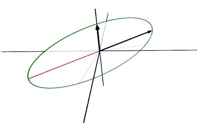
For instance, say we set the largest singular value, 3, to 0. We then get this matrix:

\[ A_1 = \begin{bmatrix} \frac{\sqrt{2}}{2} & -\frac{\sqrt{2}}{2} & 0.0 \\ \frac{\sqrt{2}}{2} & \frac{\sqrt{2}}{2} & 0.0 \\ 0 & 0 & 1 \end{bmatrix} \begin{bmatrix} 0 & 0 & 0 \\ 0 & 2 & 0 \\ 0 & 0 & 1 \end{bmatrix} \begin{bmatrix} 1 & 0 & 0 \\ 0 & 1 & 0 \\ 0 & 0 & 1 \end{bmatrix} = \begin{bmatrix} 0 & -\frac{\sqrt{2}}{2} & 0 \\ 0 & \frac{\sqrt{2}}{2} & 0 \\ 0 & 0 & 1 \end{bmatrix} \]

which transforms the unit sphere like this:

The resulting figure now lives in a 2-dimensional space. Further, the largest singular value of \(A_1\) is now 2. Set it to 0:

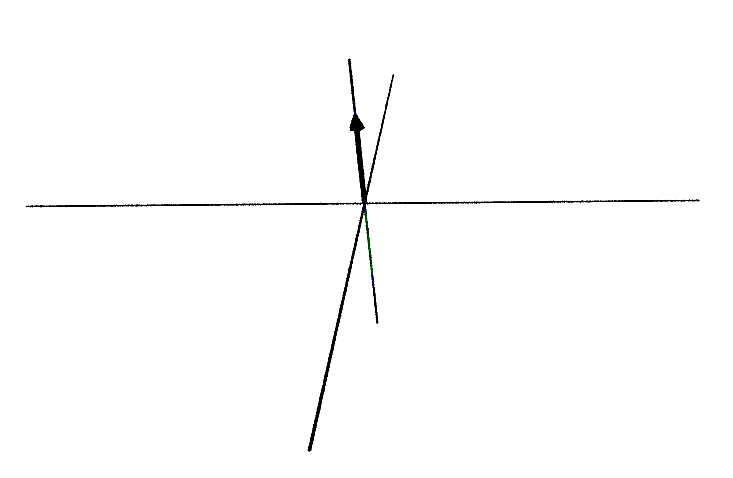
\[ A_2 = \begin{bmatrix} \frac{\sqrt{2}}{2} & -\frac{\sqrt{2}}{2} & 0.0 \\ \frac{\sqrt{2}}{2} & \frac{\sqrt{2}}{2} & 0.0 \\ 0 & 0 & 1 \end{bmatrix} \begin{bmatrix} 0 & 0 & 0 \\ 0 & 0 & 0 \\ 0 & 0 & 1 \end{bmatrix} \begin{bmatrix} 1 & 0 & 0 \\ 0 & 1 & 0 \\ 0 & 0 & 1 \end{bmatrix} = \begin{bmatrix} 0 & 0 & 0 \\ 0 & 0 & 0 \\ 0 & 0 & 1 \end{bmatrix} \]

And we get a 1-dimensional figure, and a final largest singular value of 1:

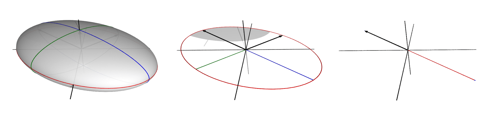
This is the point: Each set of singular vectors will form an orthonormal basis for some linear subspace of \(\mathbb{R}^n\). A singular value and its singular vectors give the direction of maximum action among all directions orthogonal to the singular vectors of any larger singular value.

This has important applications. There are many problems in statistics and machine learning that come down to finding a low-rank approximation to some matrix at hand. Principal component analysis is a problem of this kind. It says: approximate some matrix \(X\) of observations with a number of its uncorrelated components of maximum variance. This problem is solved by computing its singular value decomposition and setting some of its smallest singular values to 0.

, , ,
Published: November 12, 2019

Introduction

Say \(V\) and \(W\) are vector spaces with scalars in some field \(\mathbb{F}\) (the real numbers, maybe). A linear map is a function \(T : V \rightarrow W \) satisfying two conditions:

  • additivity \(T(x + y) = T x + T y\) for all \(x, y \in V\)
  • homogeneity \(T(c x) = c (T x)\) for all \(c \in \mathbb{F} \) and all \(x \in V\)

Defining a linear map this way just ensures that anything that acts like a vector in \(V\) also acts like a vector in \(W\) after you map it over. It means that the map preserves all the structure of a vector space after it’s applied.

It’s a simple definition – which is good – but doesn’t speak much to the imagination. Since linear algebra is possibly the most useful and most ubiquitous of all the branches of mathematics, we’d like to have some intuition about what linear maps are so we have some idea of what we’re doing when we use it. Though not all vectors live there, the Euclidean plane \(\mathbb{R}^2\) is certainly the easiest to visualize, and the way we measure distance there is very similar to the way we measure error in statistics, so we can feel that our intuitions will carry over.

It turns out that all linear maps in \(\mathbb{R}^2\) can be factored into just a few primitive geometric operations: scaling, rotation, and reflection. This isn’t the only way to factor these maps, but I think it’s the easiest to understand. (We could get by without rotations, in fact.)

Three Primitive Transformations

Scaling

A (non-uniform) scaling transformation \(D\) in \(\mathbb{R}^2\) is given by a diagonal matrix:

\[Scl(d1, d2) = \begin{bmatrix} d_1 & 0 \\ 0 & d_2 \\ \end{bmatrix}\]

where \(d_1\) and \(d_2\) are non-negative. The transformation has the effect of stretching or shrinking a vector along each coordinate axis, and, so long as \(d_1\) and \(d_2\) are positive, it will also preserve the orientation of vectors after mapping because in this case \(\det(D) = d_1 d_2 > 0\).

For instance, here is the effect on a vector of this matrix: \[D = \begin{bmatrix} 0.75 & 0 \\ 0 & 1.25 \\ \end{bmatrix}\]

It will shrink a vector by a factor of 0.75 along the x-axis and stretch a vector by a factor of 1.25 along the y-axis.

If we think about all the vectors of length 1 as being the points of the unit circle, then we can get an idea of how the transformation will affect any vector. We can see a scaling as a continous transformation beginning at the identity matrix.

If one of the diagonal entries is 0, then it will collapse the circle on the other axis.

\[D = \begin{bmatrix} 0 & 0 \\ 0 & 1.25 \\ \end{bmatrix}\]

This is an example of a rank-deficient matrix. It maps every vector onto the y-axis, and so its image has a dimension less than the dimension of the full space.

Rotation

A rotation transformation \(Ref\) is given by a matrix: \[Ref(\theta) = \begin{bmatrix} \cos(\theta) & -\sin(\theta) \\ \sin(\theta) & \cos(\theta) \\ \end{bmatrix}\]

This transformation will have the effect of rotating a vector counter-clockwise by an angle \(\theta\), when \(\theta\) is positive, and clockwise by \(\theta\) when \(\theta\) is negative.

And the unit circle gets mapped onto itself.

It shouldn’t be too hard to convince ourselves that the matrix we’ve written down is the one we want. Take some unit vector and write its coordinates like \((\cos\gamma, \sin\gamma)\). Multiply it by \(Ref(\theta)\) to get \((\cos\gamma \cos\theta - \sin\gamma \sin\theta, \cos\gamma \sin\theta + \sin\gamma \cos\theta)\). But by a trigonometric identity, this is exactly the vector \((\cos(\gamma + \theta), \sin(\gamma + \theta))\), which is our vector rotated by \(\theta\).

A rotation should preserve not only orientations, but also distances. Now, recall that the determinant for a \(2\times 2\) matrix \(\begin{bmatrix} a & b \\ c & d \end{bmatrix}\) is \(a d - b c\). So a rotation matrix will have determinant \(\cos^2(\theta) + \sin^2(\theta)\), which, by the Pythagorean identity, is equal to 1. This, together with the fact that its columns are orthonormal means that it does preserve both. It is a kind of orthogonal matrix, which is a kind of isometry.

Reflection

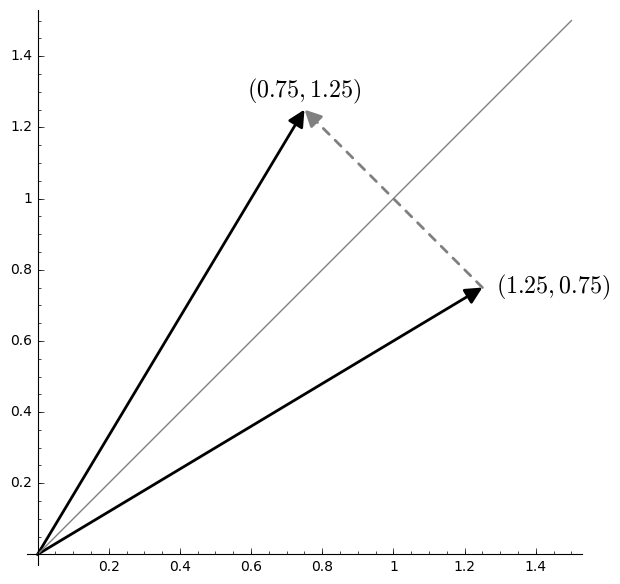
A reflection in \(\mathbb{R}^2\) can be described with matricies like: \[Ref(\theta) = \begin{bmatrix} \cos(2\theta) & \sin(2\theta) \\ \sin(2\theta) & -\cos(2\theta) \\ \end{bmatrix}\] where the reflection is through a line crossing the origin and forming an angle \(\theta\) with the x-axis.

And the unit circle gets mapped onto itself.

Note that the determinant of this matrix is -1, which means that it reverses orientation. But its columns are still orthonormal, and so it too is an isometry.

Decomposing Matricies into Primitives

The singular value decomposition (SVD) will factor any matrix \(A\) having like this:

\[ A = U \Sigma V^* \]

We are working with real matricies, so \(U\) and \(V\) will both be orthogonal matrices. This means each of these will be either a reflection or a rotation, depending on the pattern of signs in its entries. The matrix \(\Sigma\) is a diagonal matrix with non-negative entries, which means that it is a scaling transform. (The \(*\) on the \(V\) is the conjugate-transpose operator, which just means ordinary transpose when \(V\) doesn’t contain any imaginary entries. So, for us, \(V^* = V^\top\).) Now with the SVD we can rewrite any linear transformation as:

  1. \(V^*\): Rotate/Reflect
  2. \(\Sigma\): Scale
  3. \(U\): Rotate/Reflect

Example

\[\begin{bmatrix} 0.5 & 1.5 \\ 1.5 & 0.5 \end{bmatrix} \approx \begin{bmatrix} -0.707 & -0.707 \\ -0.707 & 0.707 \end{bmatrix} \begin{bmatrix} 2.0 & 0.0 \\ 0.0 & 1.0 \end{bmatrix} \begin{bmatrix} -0.707 & -0.707 \\ 0.707 & -0.707 \end{bmatrix} \]

This turns out to be:

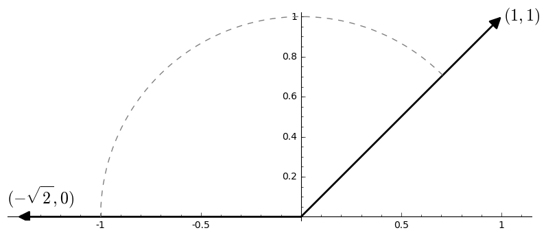
  1. \(V^*\): Rotate clockwise by \(\theta = \frac{3 \pi}{4}\).
  2. \(\Sigma\): Scale x-coordinate by \(d_1 = 2\) and y-coordinate by \(d_2 = 1\).
  3. \(U\): Reflect over the line with angle \(-\frac{3\pi}{8}\).

Example

And here is a shear transform, represented as: rotation, scale, rotation.

\[\begin{bmatrix} 1.0 & 1.0 \\ 0.0 & 1.0 \end{bmatrix} \approx \begin{bmatrix} 0.85 & -0.53 \\ 0.53 & 0.85 \end{bmatrix} \begin{bmatrix} 1.62 & 0.0 \\ 0.0 & 0.62 \end{bmatrix} \begin{bmatrix} 0.53 & 0.85 \\ -0.85 & 0.53 \end{bmatrix} \]
, , , , ,
Published: October 4, 2019

Bayesian Aggregation

Yang, Y., & Dunson, D. B., Minimax Optimal Bayesian Aggregation 2014 (arXiv)

Say we have a number of estimators \(\hat f_1, \ldots, \hat f_K\) derived from a number of models \(M_1, \ldots, M_K\) for some regression problem \(Y = f(X) + \epsilon\), but, as is the nature of things when estimating with limited data, we don’t know which estimator represents the true model (assuming the true model is in our list). The Bayesian habit is to stick a prior on the uncertainty, compute posteriors probabilities, and then average across the unknown parameter using the posterior probabilities as weights. Since the posterior probabilities (call them \(\lambda_1, \ldots, \lambda_K\)) have to sum to 1, we obtain a convex combination of our estimators \[ \hat f = \sum_{1\leq i \leq K} \lambda_i \hat f_i \] This is the approach of Bayesian Model Averaging (BMA). Yang et al. propose to find such combinations using a Dirichlet prior on the weights \(\lambda_i\). If we remove the restriction that the weights sum to 1 and instead only ask that they have finite sum in absolute value, then we obtain \(\hat f\) as a linear combination of \(\hat f_i\). The authors then place a Gamma prior on \(A = \sum_i |\lambda_i|\) and a Dirichlet prior on \(\mu_i = \frac{|\lambda_i|}{A}\). In both the linear and the convex cases they show that the resulting estimator is minimax optimal in the sense that it will give the best worst-case predictions for a given number of observations, including the case where a sparsity restriction is placed on the number of estimators \(\hat f_i\); in other words, \(\hat f\) converges to the true estimator as the number of observations increases with minimax optimal risk. The advantage to previous non-bayesian methods of linear or convex aggregation is that the sparsity parameter can be learned from the data. The Dirichlet convex combination gives good performance against Best Model selection, Majority Voting, and SuperLearner, especially when there are both a large number of observations and a large number of estimators.

I implemented the convex case in R for use with brms. The Dirichlet distribution has been reparameterized as a sum of Gamma RVs to aid in sampling. The Dirichlet concentration parameter is \(\frac{\alpha}{K^\gamma}\); the authors recommend choosing \(\alpha = 1\) and \(\gamma = 2\).

convex_regression <- function(formula, data,
                              family = "gaussian",
                              ## Yang (2014) recommends alpha = 1, gamma = 2
                              alpha = 1, gamma = 2,
                              verbose = 0,
                              ...) {
  if (gamma <= 1) {
    warning(paste("Parameter gamma should be greater than 1. Given:", gamma))
  }
  if (alpha <= 0) {
    warning(paste("Parameter alpha should be greater than 0. Given:", alpha))
  }
  ## Set up priors.
  K <- length(terms(formula))
  alpha_K <- alpha / (K^gamma)
  stanvars <-
    stanvar(alpha_K,
      "alpha_K",
      block = "data",
      scode = "  real<lower = 0> alpha_K;  // dirichlet parameter"
    ) +
    stanvar(
      name = "b_raw",
      block = "parameters",
      scode = "  vector<lower = 0>[K] b_raw; "
    ) +
    stanvar(
      name = "b",
      block = "tparameters",
      scode = "  vector[K] b = b_raw / sum(b_raw);"
    )
  prior <- prior("target += gamma_lpdf(b_raw | alpha_K, 1)",
    class = "b_raw", check = FALSE
  )
  f <- update.formula(formula, . ~ . - 1)
  if (verbose > 0) {
    make_stancode(f,
      prior = prior,
      data = data,
      stanvars = stanvars
    ) %>% message()
  }
  fit_dir <- brm(f,
    prior = prior,
    family = family,
    data = data,
    stanvars = stanvars,
    ...
  )
  fit_dir
}

Here is a gist that includes an interface to parsnip.

In my own experiments, I found the performance of the convex aggregator to be comparable to a LASSO SuperLearner at the cost of the lengthier training that goes with MCMC methods and the finicky convergence of sparse priors. So I would likely reserve this for when I had lots of features and lots of estimators to work through, where I presume it would show an advantage. But in that case it would definitely be on my list of things to try.

Bayesian Stacking

Yao, Y., Vehtari, A., Simpson, D., & Gelman, A., Using Stacking to Average Bayesian Predictive Distributions (pdf)

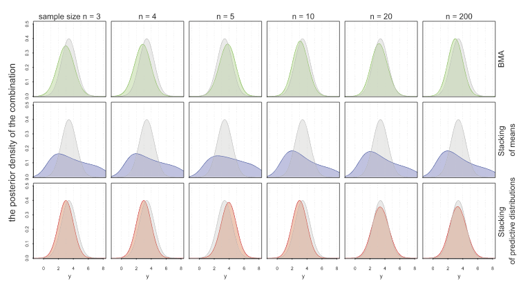
Another approach to model combination is stacking. With stacking, model weights are chosen by cross-validation to minimize RMSE predictive error. Now, BMA finds the aggregated model that best fits the data, while stacking finds the aggregated model that gives the best predictions. Stacking therefore is usually better when predictions are what you want. A drawback is that stacking produces models through point estimates. So, they don’t give you all the information of a full distribution like BMA would. Yao et al. propose a method of stacking that instead finds the optimal predictive distribution by convex combinations of distributions with weights chosen by some scoring rule: the authors use the minimization of KL-divergence. Hence, they choose weights \(w\) empirically through LOO by \[ \max_w \frac{1}{n} \sum_{1\leq i \leq n} \log \sum_{1\leq k \leq K} w_k p(y_i | y_{-i}, M_k) \] where \(y_1, \ldots, y_n\) are the observed data and \(y_{-i}\) is the data with \(y_i\) left out. The following figure shows how stacking of predictive distributions gives the “best of both worlds” for BMA and point prediction stacking.

From Yao (2018)

They have implemented stacking for Stan models in the R package loo.