numpy, sage, tensors
Published: February 5, 2019

Tensors can sometimes have a fearsome reputation. They are at heart, however, no more difficult to define than polynomials. I’ve tried in these notes to take a computational focus and to avoid formalism when possible; I haven’t assumed any more than what you might encounter in an undergraduate linear algebra course. If you’re interested in tensors applied to machine learning, or have wondered why arrays in Tensorflow are called tensors, you might find this useful. I’ll do some computations in Sage and also in Numpy for illustration.

Abstract Tensors

First, let’s take brief look at tensors in the abstract. This is just to give us an idea of what properties they have and how they function. I’ll gloss over most of the details of the construction.

A tensor is a vector. It is an element of a vector space. Being a vector, if we have a basis for the space we can write the tensor as a list of coordinates (or maybe something like a matrix or an array – we’ll see how).

A tensor is a vector in a product vector space. This means that part of it comes from one vector space and part of it comes from another. These parts combine in a way that fits with the usual notions of how products should work. Why would we want these tensors, these products of vectors? It turns out that lots of useful things are tensors. Matrices and linear maps are tensors, and so are determinants and inner products and cross products. Tensors give us power to express many useful ideas.

A simple product of vectors looks like \(v \otimes w\) and the product space looks like \(V \otimes W\), where \(V\) and \(W\) are vector spaces. The elements of \(V \otimes W\) are linear combinations of these simple products. So, a typical element of \(V \otimes W\) might look like \(v_1 \otimes w_2 + 5(v_4 \otimes w_1) + 3(v_3 \otimes w_2)\).

Again, \(V \otimes W\) is a vector space. Its vectors are called tensors. Tensors are linear combinations of simple tensors like \(v \otimes w\).

The tensor space \(V \otimes W\) is a vector space, but its vectors have some special properties given to them by \(\otimes\). This product has many of the same useful properties as products of numbers. They are:

\[ \textbf{Distributivity: } v \otimes (w_1 + w_2) = v \otimes w_1 + v \otimes w_2 \]

(Just like \(x(y + z) = xy + xz\).)

and

\[ \textbf{Scalar Multiples: } a (v \otimes w) = (av) \otimes w = v \otimes (aw) \]

(Just like \(a(xy) = (ax)y = x(ay)\).)

The tensor product also does what we expect with the zero vector, namely: \(v \otimes w = 0\) if and only if \(v = 0\) or \(w = 0\). The tensor product does not have the commutivity property however. A tensor \(v \otimes w\) doesn’t have to be the same as \(w \otimes v\). For one, the vector on the left has to come from \(V\) and the vector on the right has to come from \(W\).

Using these properties we can manipulate tensors just like we do polynomials. For instance:

\[\begin{equation} \begin{split} & 2(v_1 \otimes w_1) + 3(v_1 + v_2) \otimes w_1 \\ = & 2(v_1 \otimes w_1) + 3(v_1 \otimes w_1) + 3(v_2 \otimes w_1) \\ = & 5(v_1 \otimes w_1) + 3(v_2 \otimes w_1) \end{split} \end{equation} \]

You could think of an abstract tensor as a sort of polynomial where the odd-looking product \(\otimes\) reminds us that the \(v\) and \(w\) don’t generally commute.

Here’s an example. FiniteRankFreeModule is creating a vector space of dimension 2 over the quotients \(\mathbb Q\). A module is a kind of generalized vector space.

M = FiniteRankFreeModule(QQ, 2, name='M', start_index=1)
v = M.basis('v')
s = M.tensor((2, 0), name='s')
s[v,:] = [[1, 2], [3, 4]]
t = M.tensor((2, 0), name='t')
t[v,:] = [[5, 6], [7, 8]]
latex(s.display(v))
latex(t.display(v))
latex((s + t).display(v))

\[ s = v_{1}\otimes v_{1} + 2 v_{1}\otimes v_{2} + 3 v_{2}\otimes v_{1} + 4 v_{2}\otimes v_{2} \] \[ t = 5 v_{1}\otimes v_{1} + 6 v_{1}\otimes v_{2} + 7 v_{2}\otimes v_{1} + 8 v_{2}\otimes v_{2} \] \[ s+t = 6 v_{1}\otimes v_{1} + 8 v_{1}\otimes v_{2} + 10 v_{2}\otimes v_{1} + 12 v_{2}\otimes v_{2} \]

Construction of the Tensor Space

This is just a note on how the tensor space \(V \otimes W\) can be constructed from \(V\) and \(W\). It’s not essential to anything that follows.

Basically, we can construct \(V \otimes W\) the same way that we can construct the complex numbers from the real numbers. To get the complex numbers from the reals, we just add in some new number \(i\) to the real numbers and then define a simplification rule that says \(i^2 = -1\). To get \(V \otimes W\) from \(V\) and \(W\), we just take all linear combinations of vectors from \(V\) and vectors from \(W\) and then define the Distributivity and Scalar Multiplication rules. The formalism that does this is called a quotient space, or see here for the tensor product construction.

By constructing the space \(V \otimes W\) in the most general way possible (meaning, not adding any other rules except distribution and scalar multiplication), we ensure that any kind of space or object that has these kinds of linear or multilinear properties has a representation as a tensor, and any other kind of construction that satisfies these rules will be essentially equivalent to the tensor construction. (The property is called a universal property. It occurs all the time in mathematics and is very useful.) Tensors are the general language of linearity.

Tensors as Arrays

We can represent tensors as arrays, which is nice for doing computations.

If we have a basis for \(V\) and a basis for \(W\), then we can make a basis for \(V \otimes W\) in just the way we should expect: by taking all the products of the basis vectors. Namely, if \((e_i)\) is a basis for \(V\) and \((f_j)\) is a basis for \(W\), then \((e_i \otimes f_j)\) is a basis for \(V \otimes W\). This also means that the dimension of \(V \otimes W\) is the product of the dimensions of \(V\) and \(W\); that is, \(dim(V \otimes W) = dim(V)dim(W)\).

Recall that if we can write a vector in \(V\) as \(v = \sum a_i e_i\), then \((a_i)\) is its representation as a vector of coordinates. A tensor in \(V \otimes W\) will instead have a representation as a matrix. If \(m = dim(V)\) and \(n = dim(W)\), then this will be an \(m \times n\) matrix. If we write a tensor in terms of its basis elements as:

\[\sum_i \sum_j c_{i,j} (e_i \otimes f_j)\]

then its matrix is \([c_{i,j}]\). The subscript of \(e_i\) tells you the row and the subscript of \(f_j\) tells you the column. For example, let’s say \(V\) and \(W\) are both two-dimensional. We could write a tensor

\[(e_1 \otimes f_1) + 2(e_1 \otimes f_2) + 3(e_2 \otimes f_1) + 4(e_2 \otimes f_2)\]

as

\[\begin{bmatrix} 1 & 2 \\ 3 & 4 \\ \end{bmatrix} \]

But what if we have a vector \(v\) in \(V\) and a vector \(w\) in \(W\) and we want to find out what the matrix of \(v \otimes w\) is? This is easy too. Say \(v = \sum a_i e_i\) and \(w = \sum b_j f_j\). Then

\[v \otimes w = \sum_i \sum_j a_i b_j (e_i \otimes f_j)\]

and its matrix is \([a_i b_j]\). In other words, the entry in row \(i\) and column \(j\) will be \(a_i b_j\).

It’s easy to find this matrix using matrix multiplication. If we write our coordinate vectors as column vectors, then our tensor product becomes an outer product:

\[\color{RubineRed}v \color{black}\otimes \color{MidnightBlue}w\color{black} = \color{RubineRed}v\color{MidnightBlue} w^\mathsf{T}\]

For instance,

\[ \color{RubineRed}(1, 2, 3)\color{Black} \otimes \color{RoyalBlue}(4, 5, 6)\color{Black} = \color{RubineRed}\begin{bmatrix} 1\\ 2\\ 3 \end{bmatrix} \color{black} \color{RoyalBlue}[4, 5, 6]\color{black} = \begin{bmatrix} \color{RubineRed}1\color{black}\cdot \color{RoyalBlue}4\color{black} & \color{RubineRed}1\color{black}\cdot \color{RoyalBlue}5\color{black} & \color{RubineRed}1\color{black}\cdot \color{RoyalBlue}6\color{black} \\ \color{RubineRed}2\color{black}\cdot \color{RoyalBlue}4\color{black} & \color{RubineRed}2\color{black}\cdot \color{RoyalBlue}5\color{black} & \color{RubineRed}2\color{black}\cdot \color{RoyalBlue}6\color{black} \\ \color{RubineRed}3\color{black}\cdot \color{RoyalBlue}4\color{black} & \color{RubineRed}3\color{black}\cdot \color{RoyalBlue}5\color{black} & \color{RubineRed}3\color{black}\cdot \color{RoyalBlue}6\color{black}\end{bmatrix} =\begin{bmatrix} 4 & 5 & 6 \\ 8 & 10 & 15 \\ 12 & 15 & 18\end{bmatrix} \]

Notice the correspondence between the basis elements and the entries of the matrix in the next example.

M = FiniteRankFreeModule(QQ, 3, name='M', start_index=1)
e = M.basis('e')
v = M([-2, 9, 5], basis=e, name='v')
w = M([1, 0, -2], basis=e, name='w')
latex((v*w).display())
latex((v*w)[e,:])

\[ v\otimes w = -2 e_{1}\otimes e_{1} + 4 e_{1}\otimes e_{3} + 9 e_{2}\otimes e_{1} -18 e_{2}\otimes e_{3} + 5 e_{3}\otimes e_{1} -10 e_{3}\otimes e_{3} \\ \left(\begin{array}{rrr} -2 & 0 & 4 \\ 9 & 0 & -18 \\ 5 & 0 & -10 \end{array}\right) \]

We can extend the tensor product construction to any number of vector spaces. In this way we get multidimensional arrays. We might represent a tensor in a space \(U \otimes V \otimes W\) as a “matrix of matricies.”

\[ \left[\begin{array}{r} \left[\begin{array}{rr} c_{111} & c_{112} \\ c_{121} & c_{122} \end{array}\right] \\ \left[\begin{array}{rr} c_{211} & c_{212} \\ c_{221} & c_{222} \end{array}\right] \end{array}\right] \]

And we use the more general Kronecker product to find the product of tensors:

\[ \color{RubineRed}(1, 2) \color{Black} \otimes \color{RoyalBlue} \left[\begin{array}{rr} 1 & 2 \\ 3 & 4 \end{array}\right] \color{Black} = \color{RubineRed} \left[\begin{array}{r} 1 \\ 2 \end{array}\right] \color{RoyalBlue} \left[\begin{array}{rr} 1 & 2 \\ 3 & 4 \end{array}\right] \color{Black} = \left[\begin{array}{r} \color{RubineRed} 1 \color{RoyalBlue} \left[\begin{array}{rr} 1 & 2 \\ 3 & 4 \end{array}\right] \\ \color{RubineRed} 2 \color{RoyalBlue} \left[\begin{array}{rr} 1 & 2 \\ 3 & 4 \end{array}\right] \color{Black}\end{array}\right] = \left[\begin{array}{r} \left[\begin{array}{rr} 1 & 2 \\ 3 & 4 \end{array}\right] \\ \left[\begin{array}{rr} 2 & 4 \\ 6 & 8 \end{array}\right] \color{Black}\end{array}\right] \]

M = FiniteRankFreeModule(QQ, 2, name='M', start_index=1)
e = M.basis('e')
u = M([1, 2], basis=e, name='u')
vw = M.tensor((2, 0), name='vw')
vw[e,:] = [[1, 2], [3, 4]]
(u*vw).display(e)
print()
(u*vw)[e,:]
u*vw = e_1*e_1*e_1 + 2 e_1*e_1*e_2 + 3 e_1*e_2*e_1 + 4 e_1*e_2*e_2 + 2 e_2*e_1*e_1 + 4 e_2*e_1*e_2 + 6 e_2*e_2*e_1 + 8 e_2*e_2*e_2

[[[1, 2], [3, 4]], [[2, 4], [6, 8]]]

The number of vector spaces in the product space is the same as the number of dimensions in the arrays of its tensors (that is, the number of indices needed to specify a component). This number is called the “order” of a tensor (or sometimes “degree”). The order of the tensor above is 3.

We can extend this product to tensors of any order. The components of a tensor \(s \otimes t\) can always be found by taking the product of the respective components of \(s\) and \(t\). For instance, if \(s_{12} = 5\) and \(t_{345} = 7\), then \((s \otimes t)_{12345} = s_{12}t_{345} = 5\cdot7 = 35\).

M = FiniteRankFreeModule(QQ, 5, name='M', start_index=1)
e = M.basis('e')
s = M.tensor((2, 0), name='s')
s[e,1,2] = 5
t = M.tensor((3, 0), name='t')
t[e,3,4,5] = 7
(s*t)[e,1,2,3,4,5]
35

Tensors as Maps

I mentioned earlier that things like cross-products and determinants are tensors. We’ll see how that works now. Recall that every vector space \(V\) has a dual vector space \(V^*\) which is the space of all linear maps \(V \rightarrow F\), where \(F\) is the field of scalars of \(V\). In terms of matricies, we might think of elements in \(V\) as column vectors and elements of \(V^*\) as row vectors. Then, we can apply an element of \(V^*\) to an element of \(V\) just like we do when representing linear maps as matricies:

\[ \left[a_1, a_2, a_3\right] \left[\begin{array}{r} b_1 \\ b_2 \\ b_3 \end{array}\right] = a_1b_1 + a_2b_2 + a_3b_3 \]

This in fact is just the dot product of the two vectors.

Let’s take a product \(T = V \otimes \cdots \otimes V \otimes V^* \otimes \cdots \otimes V^*\). The number of times \(V\) occurs is called the “contravariant” order of the space and the number of times \(V^*\) occurs is called the “covariant” order of the space. (The reason for these names is related to the change-of-basis on vectors of those types). We say that a tensor has “type \((k, l)\)” when it is of contravariant order \(k\) and covariant order \(l\). So when we had earlier M.tensor((2, 0), name='t'), the (2, 0) was saying that we wanted a tensor with 2 contravariant parts.

Tensors of order \((0, 1)\) are mappings \(V \rightarrow F\). They will map tensors of order \((1, 0)\) (that is, column vectors) to the scalar field, and like above, this will just be the dot product of the two vectors.

M = FiniteRankFreeModule(QQ, 3, name='M', start_index=1)
e = M.basis('e')

s = M.tensor((0, 1), name='s')
s[e, :] = [1, 2, 3]
t = M.tensor((1, 0), name='t')
t[e, :] = [4, 5, 6]

v = vector([1, 2, 3])
w = vector([4, 5, 6])

s(t) == v.dot_product(w)
True

Expanding this idea, we can think of a tensor \(t\) of order \((1,1)\) either as a multilinear form \(t:V^* \otimes V \rightarrow F\) or as a linear map, as \(t:V \rightarrow V\) or as \(t:V^* \rightarrow V^*\). The difference is just in what and how many arguments we pass in to the tensor. For instance, if we pass a column vector \(v\) into the tensor \(t\) in its second position (the position of \(V\)), then we get a map \(V \rightarrow V\); this is the same as multiplying a vector by a matrix representing a linear map. This partial application is called a “contraction.”

s = M.tensor((1, 1), name='s')
s[e, :] = [[1, 2, 3], [4, 5, 6], [7, 8, 9]]
t = M.tensor((1, 0), name='t')
t[e, :] = [4, 5, 6]

m = Matrix([[1, 2, 3], [4, 5, 6], [7, 8, 9]])
w = vector([4, 5, 6])

s.contract(t)[e,:] == list(m*w)
True

Generally, we can represent any kind of multilinear map \(V^* \times \cdots \times V^* \times V \times \cdots \times V \rightarrow F\) as a tensor in the space \(V \otimes \cdots \otimes V \otimes V^* \otimes \cdots \otimes V^*\). Since determinants and cross-products are multilinear maps, they too are tensors.

Sage makes a distinction between contravariant and covariant parts, but libraries like numpy and tensorflow do not. When using these, we can contract one tensor with another along any axes whose dimensions are the same. Their contraction operation is called tensordot.

import numpy as np

s = np.ones((2, 3, 4, 5))
t = np.ones((5, 4, 3, 2))
np.tensordot(s, t, axes=[[0, 1, 2], [3, 2, 1]])
array([[24., 24., 24., 24., 24.],
       [24., 24., 24., 24., 24.],
       [24., 24., 24., 24., 24.],
       [24., 24., 24., 24., 24.],
       [24., 24., 24., 24., 24.]])

We could think of the axes in s as representing row vectors (\(V^*\)) and the axes in t as representing column vectors (\(V\)).

We could also do this using Einstein notation. Basically, whenever an index appears twice in an expression, it means to sum over that index while multiplying together the respective components (just like a dot product on those two axes).

s = np.ones((2, 3, 4))
t = np.ones((4, 3, 2))

np.einsum('ija, bji -> ab', s, t)
array([[6., 6., 6., 6.],
       [6., 6., 6., 6.],
       [6., 6., 6., 6.],
       [6., 6., 6., 6.]])

Einstein summations are a convenient way to do lots of different kinds of tensor computations. Here are a bunch of great examples.

Conclusion

That’s all for now! For anyone reading, I hope you found it informative. Tensors can be hard to get started on, but once you see the idea, I think you’ll find them a pleasure to work with.
MCMC, NLP, data-science, bayesian, python
Published: January 30, 2019

Imagine we have some collection of documents. They could be novels, or tweets, or financial reports—just any collection of text. We want an algorithm that can discover what they are about, and we would like our algorithm to do it automatically, without any hints. (That is, we want our algorithm to be unsupervised.) We will look at several models that probabilistically assign words to topics using Bayes’ Theorem. They are all Bayesian Graphical Models.

The basic problem in statistics is to infer some unobservable value from observable instances of it. In our case, we want to infer the topics of a document from the actual words in the document. We want to be able to infer that our document is about “colors” if we observe “red” and “green” and “blue”.

Bayes’ Theorem allows us to do this. It allows us to infer probabilities concerning the unobserved value from the observations that we can make. It allows us to reason backwards in some sense. So, when constructing a Bayesian model, it is helpful to think backwards. Instead of first asking how words are distributed to topics and topics to documents, we will ask how we could generate a document if we already knew these distributions. To construct our model, we will first reason from the unknown values to the known values so that we know how to do the converse when the time comes.

Some Simple Generative Examples

In all of our models, we are going make a simplfying assumption. We will assume that all of the words in a document occur independently of whatever words came before or come after; that is, a document will just be a “bag of words.” We’ll see that even with ignoring word-order, we can still infer pretty accurately what a document might be about.

Let’s start with a very simple example: 1 document with 1 topic and 2 words in our vocabulary.

(Some definitions: The “vocabulary” is just the set of unique words that occur in all of the documents together, the “corpus.” We’ll refer to a word in the vocabulary as just a “word” and some instance of a word in a document as a “token.”)

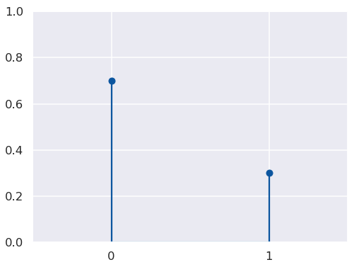
Let’s say our two words are “blue” and “red”, and that the probability of any given word (any token) being “red” is \(\phi\): \(P(W = red) = \phi\). This is the same as saying our random variable of tokens \(W\) has a Bernoulli distribution with parameter \(\phi\): \(W \sim Bernoulli(\phi)\).

The distribution looks like this:

x = [0, 1]
pmf = st.bernoulli.pmf(x, 0.3)

plt.stem(x, pmf)
plt.xticks([0,1])
plt.ylim(0,1)
plt.xlim(-0.5, 1.5)
(-0.5, 1.5)
Bernoulli pmf

Here, 1 represents “red” and 0 represents “blue” (or not-“red”).

And here is how we could generate a document with this model:

coding = {0 : "blue", 1 : "red"}
W = 50  # number of tokens in the document
tokens = st.bernoulli.rvs(0.3, size = W)  # choose the tokens
print(' '.join(str(w) for w in [coding[i] for i in tokens]))
blue blue red blue red blue blue red red blue blue blue blue blue blue blue blue red blue blue blue blue blue blue blue blue blue red red blue blue blue blue blue blue red blue blue red blue red blue red blue blue blue blue blue red blue

Unigram Model

For the general model, we will also choose the distribution of words within the topic randomly. That is, we will assign a probability distribution to \(\phi\).

The beta distribution is a natural choice. Since its support is \([0,1]\) it can represent randomly chosen probabilities (values between 0 and 1). It is also conceptually convenient being the conjugate prior of the Bernoulli distribution, which allows us to make a more explicit connection between its parameters and the parameters of its Bernoulli distribution.

The model is now:

\(\phi \sim Beta(\beta_0, \beta_1)\)

\(W \sim Bernoulli(\phi)\)

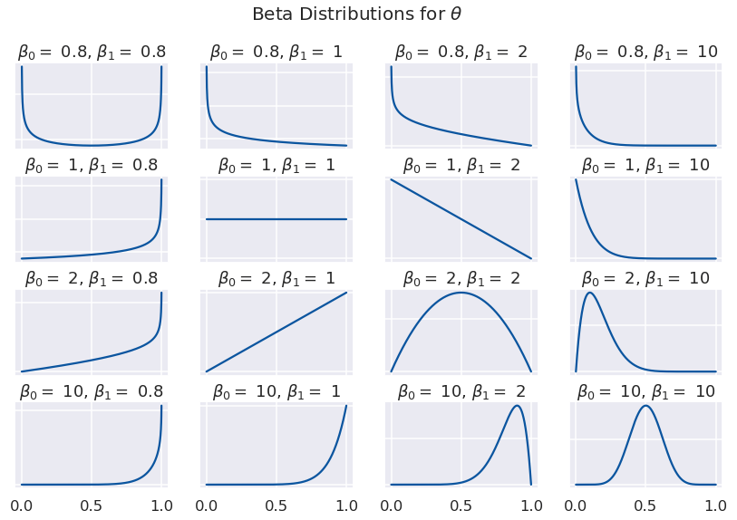
where \(\beta_0\) and \(\beta_1\) are the “shape parameters” of the beta distribution. We can think of them as the assumed counts of each word, or the “pseudo-counts.” Let’s see how different values of these parameters affect the shape of the distribution.

beta_0 = [0.8, 1, 2, 10]
beta_1 = [0.8, 1, 2, 10]

x = np.array(np.linspace(0, 1, 1000))

f, axarr = plt.subplots(len(beta_0), len(beta_1), sharex='all', sharey='none')

for i in range(len(beta_0)):
    for j in range(len(beta_1)):
        a = beta_0[i]
        b = beta_1[j]
        y = st.beta(a, b).pdf(x)
        axarr[i, j].plot(x, y)
        axarr[i, j].axes.yaxis.set_ticklabels([])
        axarr[i, j].set_title(r'$\beta_0 =$ ' + str(a) + r', $\beta_1 =$ ' + str(b))

f.subplots_adjust(hspace=0.3)
f.suptitle(r'Beta Distributions for $\theta$', fontsize=20)
Text(0.5, 0.98, 'Beta Distributions for $\\theta$')
a grid of six beta pdfs for various parameters

Values near 0 will favor “blue” and values near 1 will favor “red”. We can choose \(\beta_0\) and \(\beta_1\) to generate the kinds of documents we like. (The notation is a bit backwards here: \(\beta_0\) is the pseudo-count for “red”, whose probability is toward 1, on the right of the graph. So \(\beta_0 > \beta_1\) means more “red”s, and vice versa.)

Let’s generate some documents with this expanded model. We’ll set \(\beta_0 = 0.8\) and \(\beta_1 = 0.8\). We would expect most of our documents to favor one word or the other, but overall to occur equally often.

beta_0 = 0.8
beta_1 = 0.8

thetas = st.beta.rvs(beta_0, beta_1, size = 6)

W = 10  # number of tokens in each document

for t in thetas:
    print('Theta: ', t)
    tokens = st.bernoulli.rvs(t, size = W)
    print('Document: ' + ' '.join(str(w) for w in [coding[i] for i in tokens]) + '\n')
Theta:  0.2376299911870814
Document: blue red blue blue red red blue blue blue blue

Theta:  0.768902025579346
Document: red red red red blue red red red blue red

Theta:  0.6339386112711662
Document: red blue red blue red blue blue blue red blue

Theta:  0.889248394241369
Document: red red red blue red red red red red red

Theta:  0.7522981849896823
Document: red red red red blue blue red red red red

Theta:  0.18416659985533126
Document: blue red red blue blue blue red red blue blue

(We could also assign a distribution to W, the number of tokens in each document. (Blei 2003) uses a Poisson distribution.)

Let’s look at a couple more.

Mixture of Unigrams

Here, we’ll also choose a single topic for each document, from among two. To simplify things, we’ll also assume the topics generate distinct words and that the proportions of words in topics are similar, that is, that they have the same shape parameters. We’ll see later that is a good assumption when using inference models.

Distribution of topics to documents: \(\theta \sim Beta(\alpha_0, \alpha_1)\)

Distribution of words to Topic 0: \(\phi_0 \sim Beta(\beta_0, \beta_1)\)

Distribution of words to Topic 1: \(\phi_1 \sim Beta(\beta_0, \beta_1)\)

The topics: \(T \sim Bernoulli(\theta)\)

Words from Topic 0: \(W_1 \sim Bernoulli(\phi_0)\)

Words from Topic 1: \(W_2 \sim Bernoulli(\phi_1)\)

coding_0 = {0:'blue', 1:'red'}  # words in topic 0
coding_1 = {0:'dogs', 1:'cats'}  # words in topic 1

D = 15  # number of documents in corpus
W = 10  # number of tokens in each document

alpha_0, alpha_1 = 1, 1.5
beta_0, beta_1 = 0.8, 0.8

theta = st.beta.rvs(alpha_0, alpha_1, size = 1)[0]  # choose a distribution of topics to documents
phi_0 = st.beta.rvs(beta_0, beta_1, size = 1)[0] # choose distribution of words in topic 0
phi_1 = st.beta.rvs(beta_0, beta_1, size = 1)[0] # choose distribution of words in topic 1

topics = st.bernoulli.rvs(theta, size = D)  # choose a topic for each document

print('Theta: {:.3f}  Phi_0: {:.3f}  Phi_1: {:.3f}'.format(theta, phi_0, phi_1))
for i in range(D):
    if topics[i] == 0:
        tokens = st.bernoulli.rvs(phi_0, size = W)
        print('Document: ' + ' '.join(str(w) 
              for w in [coding_0[i] for i in tokens]))
    else:
        tokens = st.bernoulli.rvs(phi_1, size = W)
        print('Document: ' + ' '.join(str(w) 
              for w in [coding_1[i] for i in tokens]))
Theta: 0.114  Phi_0: 0.973  Phi_1: 0.637
Document: red red red red red red red red red red
Document: red red red blue red red red red red red
Document: red red red red red red red red red red
Document: dogs dogs cats cats cats cats cats dogs cats dogs
Document: red red red red red red red red red red
Document: red red blue red red red red red red red
Document: red red red red red red red red red red

Latent Dirichlet Allocation

This time, instead of choosing a single topic for each document, we’ll choose a topic for each word. This will make our model much more flexible and its behavior more realistic.

Distribution of topics within documents: \(\theta \sim Beta(\alpha_0, \alpha_1)\)

Distribution of words to Topic 0: \(\phi_0 \sim Beta(\beta_0, \beta_1)\)

Distribution of words to Topic 1: \(\phi_1 \sim Beta(\beta_0, \beta_1)\)

The topics: \(T \sim Bernoulli(\theta)\)

Words from Topic 0: \(W_1 \sim Bernoulli(\phi_0)\)

Words from Topic 1: \(W_2 \sim Bernoulli(\phi_1)\)

coding_0 = {0:'blue', 1:'red'}  # words in topic 0
coding_1 = {0:'dogs', 1:'cats'}  # words in topic 1

D = 15
W = 10  # number of tokens in each document

alpha_0, alpha_1 = 1, 1.5
beta_0, beta_1 = 0.8, 0.8

theta = st.beta.rvs(alpha_0, alpha_1, size = 1)[0]  # choose a distribution of topics to documents
phi_0 = st.beta.rvs(beta_0, beta_1, size = 1)[0]  # choose distribution of words in topic 0
phi_1 = st.beta.rvs(beta_0, beta_1, size = 1)[0]  # choose distribution of words in topic 1

print('Theta: {:.3f}  Phi_0: {:.3f}  Phi_1: {:.3f}'.format(theta, phi_0, phi_1))
for i in range(D):
    print('Document: ', end='')
    topics = st.bernoulli.rvs(theta, size=W)  # choose topics for each word
    for j in range(W):
        if topics[j] == 0:
            token = st.bernoulli.rvs(phi_0, size=1)[0]  # choose a word from topic 0
            print(coding_0[token], end=' ')
        else:
            token = st.bernoulli.rvs(phi_1, size=1)[0]  # choose a word from topic 1
            print(coding_1[token], end=' ')
    print() 
Theta: 0.384  Phi_0: 0.127  Phi_1: 0.028
Document: dogs blue blue blue dogs blue dogs blue blue blue 
Document: blue dogs blue blue dogs dogs dogs dogs blue cats 
Document: blue dogs blue blue blue dogs red dogs blue blue 
Document: dogs dogs red dogs dogs blue dogs blue blue blue 
Document: blue dogs dogs blue blue dogs red dogs dogs red 
Document: dogs blue blue red dogs blue dogs blue blue blue 
Document: blue blue blue dogs blue dogs blue dogs dogs blue 
Document: dogs red dogs red dogs blue dogs dogs blue blue 
Document: dogs dogs blue dogs blue dogs blue blue blue dogs 
Document: dogs blue blue blue blue red blue blue dogs dogs 
Document: dogs dogs blue red dogs dogs blue blue blue blue 
Document: blue blue blue red dogs blue blue blue blue red 
Document: blue blue blue dogs blue dogs red dogs blue dogs 
Document: dogs blue blue dogs dogs dogs blue dogs dogs blue 
Document: dogs dogs dogs red blue dogs red dogs dogs dogs 

The Dirichlet Distribution

Before we go on, we need to generalize our model a bit to be able to handle arbitrary numbers of words and topics, instead of being limited to just two. The multivariate generalization of the Bernoulli distribution is the categorical distribution, which simply gives a probability to each of some number of categories. The generalization of the beta distribution is a little trickier. It is called the Dirichlet distribution. And just like samples from the beta distribution will give parameters for a Bernoulli RV, samples from the Dirichlet distribution will give parameters for the categorical RV.

Let’s recall the two requirements for some set of \(p\)’s to be probability parameters to a categorical distribution. First, they have to sum to 1: \(p_0 + p_1 + \cdots + p_v = 1\). This means they form a hyperplane in \(v\)-dimensional space. Second, they all have to be non-negative: \(p_i \geq 0\). This means they all lie in the first quadrant (or orthant, more precisely). The geometric object that satisfies these two requirements is a simplex. In the case of two variables it will be a line-segment and in the case of three variables it will be a triangle.

As sampled from the distribution, these values will form barycentric coordinates on the simplex. This just means that the coordinates tell you how far the point is from the center of the simplex, instead of how far it is from the origin, like with Cartesian coordinates.

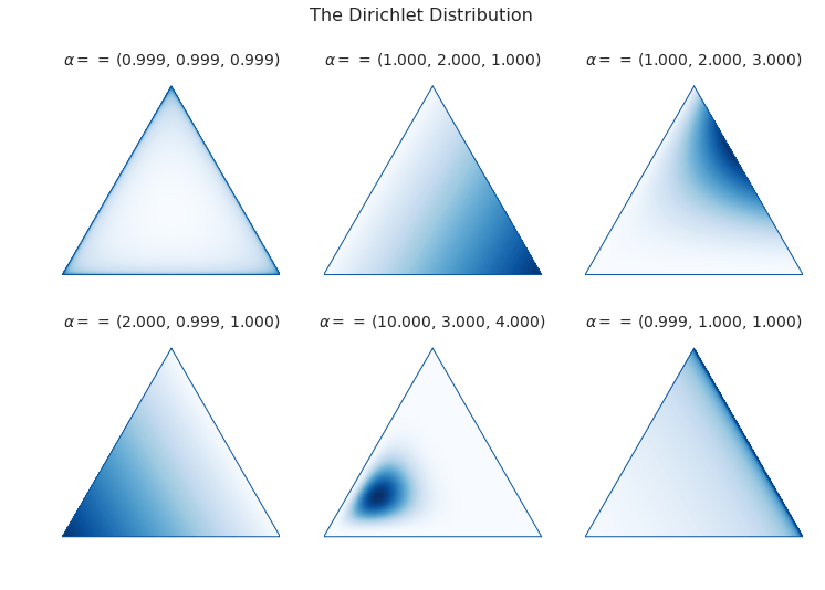
The 3-dimensional Dirichlet returns barycentric coordinates on the 2-simplex, a triangle. We can visualize the surface of the Dirichlet pdf as existing over a triangle; that is, its domain is the simplex.

import simplex_plots as sp
# from https://gist.github.com/tboggs/8778945

alphas = [[0.999, 0.999, 0.999], [1, 2, 1], [1, 2, 3], 
          [2, 0.999, 1], [10, 3, 4], [0.999, 1, 1]]

fig = plt.figure(figsize=(12, 8))
fig.suptitle('The Dirichlet Distribution', fontsize=16)
for i, a in enumerate(alphas):
    plt.subplot(2, len(alphas)/2, i + 1)
    sp.draw_pdf_contours(sp.Dirichlet(a), border=True, cmap='Blues')
    title = r'$\alpha = $ = ({0[0]:.3f}, {0[1]:.3f}, {0[2]:.3f})'.format(a)
    plt.title(title, fontdict={'fontsize': 14})
various dirichlet pdfs

Each corner of the triangle will favor a particular category (a word or a topic), just like either side of the domain of the beta distribution favored a category.

As in the upper left picture, whenever all of the entries in \(\alpha\) are equal, we call the distribution “symmetric,” and whenever they are all less then 1, we call the distribution “sparse.” Distributions that are both symmetric and sparse are often used as priors when inferring a topic model, symmetry because we don’t a priori have any reason to favor one unknown category over another, and sparsity to encourage our categories to be distinct.

Now let’s start developing our models.

The Full Model

Data Preparation

First we’ll make up a corpus and put it into an encoding that our models can use. To simplify things, we’ll let all of our documents have the same number of tokens and flatten the encoded data structure.

from sklearn.preprocessing import LabelEncoder
from sklearn.feature_extraction.text import CountVectorizer

corpus = [
    'Red blue green. Green blue blue? Red, red, blue, yellow.',
    'Car light red stop. Stop car. Car drive green, yellow.',
    'Car engine gas stop! Battery engine drive, car. Electric, gas.',
    'Watt, volt, volt, amp. Battery, watt, volt, electric volt charge. ',
]

tokenizer = CountVectorizer(lowercase=True).build_analyzer()
encoder = LabelEncoder()

corpus_tokenized = np.array([tokenizer(doc) for doc in corpus])  # assign a number to each word
encoder.fit(corpus_tokenized.ravel())
vocab = list(encoder.classes_)  # the vocabulary

# The number of documents and their length
D, W = corpus_tokenized.shape
# The number of words in the vocabulary
V = len(vocab)

# Flatten and encode the corpus, and create an index.
data = corpus_tokenized.ravel()
data = encoder.transform(data)
data_index = np.repeat(np.arange(D), W)

Now a couple of diagnostic functions.

def print_top_words(vocab, phis, n):
    '''Prints the top words occuring within a topic.'''
    for i, p in enumerate(phis):
        z = list(zip(vocab, p))
        z.sort(key = lambda x: x[1], reverse=True)
        z = z[0:n]

        for word, percent in z:
            print(f'Topic: {i:2}  Word: {word:10}  Percent: {percent:0.3f}')

        print()

def print_corpus_topics(corpus_tokenized, zs):
    '''Prints the corpus together with the topic assigned to each word.'''
    for d in range(zs.shape[0]):  # the document index
        for w in range(zs.shape[1]):  # the word index
            print(f'({corpus_tokenized[d, w]}, {zs[d, w]})', end=' ')
        print('\n')

The Unigram Model

In this model, words from every document are drawn from a single categorical distribution.

Distribution of words in a document: \(\phi \sim Dir(\vec{\beta})\), where \(\vec{\beta}\) is a vector of shape parameters

Distribution of tokens: \(W \sim Cat(\vec{\phi})\)

Markov-Chain Monte Carlo is a technique for sampling a model to discover its posterior parameters statistically. When models become complex, it is often the case that analytic solutions for the parameters are intractable. We will use the PyMC3 package.

First we describe the model.

# Pseudo-counts for each vocab word occuring in the documents.
beta = np.ones(V)

with pm.Model() as unigram_model:

    # Distribution of word-types in the corpus.
    phi = pm.Dirichlet('phi', a = beta)

    # The distribution of words.
    w = pm.Categorical('w', p = phi, observed = data)

Next we sample the model to create the posterior distribution.

with unigram_model:
    draw = 5000
    unigram_trace = pm.sample(5000, tune=1000, chains=4, progressbar=False)

And now we can see what the model determined the proportion of each word in the corpus was.

print_top_words(vocab, [unigram_trace.get_values('phi')[draw-1]], len(vocab))
Topic:  0  Word: red         Percent: 0.150
Topic:  0  Word: watt        Percent: 0.145
Topic:  0  Word: car         Percent: 0.117
Topic:  0  Word: green       Percent: 0.080
Topic:  0  Word: battery     Percent: 0.073
Topic:  0  Word: volt        Percent: 0.068
Topic:  0  Word: yellow      Percent: 0.067
Topic:  0  Word: drive       Percent: 0.059
Topic:  0  Word: electric    Percent: 0.054
Topic:  0  Word: gas         Percent: 0.053
Topic:  0  Word: stop        Percent: 0.048
Topic:  0  Word: blue        Percent: 0.030
Topic:  0  Word: engine      Percent: 0.025
Topic:  0  Word: charge      Percent: 0.021
Topic:  0  Word: light       Percent: 0.011
Topic:  0  Word: amp         Percent: 0.002

Mixture of Unigrams (Naive Bayes)

In this model, each document is assigned a topic and each topic has its own distribution of words.

Distribution of topics to documents: \(\vec{\theta} \sim Dirichlet(\vec{\alpha})\)

Distribution of words to topics: \(\vec{\phi} \sim Dirichlet(\vec{\beta})\)

The topics: \(T \sim Categorical(\vec{\theta})\)

The tokens: \(W \sim Categorical(\vec{\phi})\)

# Number of topics    
K = 3

# Pseudo-counts for topics and words.
alpha = np.ones(K)*0.8
beta = np.ones(V)*0.8

with pm.Model() as naive_model:
    # Global topic distribution
    theta = pm.Dirichlet("theta", a=alpha)

    # Word distributions for K topics
    phi = pm.Dirichlet("phi", a=beta, shape=(K, V))

    # Topic of documents
    z = pm.Categorical("z", p=theta, shape=D)

    # Words in documents
    p = phi[z][data_index]
    w = pm.Categorical("w", p=p, observed=data)
with naive_model:
    draw = 5000
    naive_trace = pm.sample(draw, tune=1000, chains=4, progressbar=False)
print_top_words(vocab, naive_trace['phi'][draw-1], 5)
Topic:  0  Word: drive       Percent: 0.177
Topic:  0  Word: car         Percent: 0.166
Topic:  0  Word: red         Percent: 0.126
Topic:  0  Word: blue        Percent: 0.108
Topic:  0  Word: green       Percent: 0.086

Topic:  1  Word: car         Percent: 0.238
Topic:  1  Word: green       Percent: 0.192
Topic:  1  Word: watt        Percent: 0.180
Topic:  1  Word: blue        Percent: 0.070
Topic:  1  Word: red         Percent: 0.045

Topic:  2  Word: volt        Percent: 0.161
Topic:  2  Word: car         Percent: 0.123
Topic:  2  Word: engine      Percent: 0.113
Topic:  2  Word: electric    Percent: 0.094
Topic:  2  Word: gas         Percent: 0.081

Latent Dirichlet Allocation

In this model, each word is assigned a topic and topics are distributed varyingly within each document.

Distribution of topics within documents: \(\vec{\theta} \sim Dirichlet(\vec{\alpha})\)

Distribution of words to topics: \(\vec{\phi} \sim Dirichlet(\vec{\beta})\)

The topics: \(T \sim Categorical(\vec{\theta})\)

The tokens: \(W \sim Categorical(\vec{\phi})\)

# Number of topics    
K = 3

# Pseudo-counts. Sparse to encourage separation.
alpha = np.ones((1, K))*0.5
beta = np.ones((1, V))*0.5

with pm.Model() as lda_model:
    # Distribution of topics within each document
    theta = pm.Dirichlet("theta", a=alpha, shape=(D, K))

    # Distribution of words within each topic
    phi = pm.Dirichlet("phi", a=beta, shape=(K, V))

    # The topic for each word
    z = pm.Categorical("z", p=theta, shape=(W, D))

    # Words in documents
    p = phi[z].reshape((D*W, V))
    w = pm.Categorical("w", p=p, observed=data)
with lda_model:
    draw = 5000
    lda_trace = pm.sample(draw, tune=1000, chains=4, progressbar=False)

print_top_words(tokens, lda_trace.get_values('phi')[draw-1], 4)

At the cost of some complexity, we can rewrite our model to handle a corpus with documents of varying lengths.

alpha = np.ones([D, K])*0.5  # prior weights for the topics in each document (pseudo-counts)
beta  = np.ones([K, V])*0.5  # prior weights for the vocab words in each topic (pseudo-counts)

sequence_data = np.reshape(np.array(data), (D,W))
N = np.repeat(W, D)  # this model needs a list of document lengths

with pm.Model() as sequence_model:

    # distribution of the topics occuring in a particular document
    theta   = pm.Dirichlet('theta', a=alpha, shape=(D, K))

    # distribution of the vocab words occuring in a particular topic
    phi     = pm.Dirichlet('phi', a=beta, shape=(K, V))

    # the topic for a particular word in a particular document: shape = (D, N[d])
    # theta[d] is the vector of category probabilities for each topic in 
    # document d.
    z = [pm.Categorical('z_{}'.format(d), p = theta[d], shape=N[d])
          for d in range(D)]

    # the word occuring at position n, in a particular document d: shape = (D, N[d]) 
    # z[d] is the vector of topics for document d
    # z[d][n] is the topic for word n in document d
    # phi[z[d][n]] is the distribution of words for topic z[d][n]
    # [d][n] is the n-th word observed in document d
    w = [pm.Categorical('w_{}_{}'.format(d, n), p=phi[z[d][n]],
                        observed = sequence_data[d][n])
         for d in range(D) for n in range(N[d])]

with sequence_model:
    draw = 5000
    sequence_trace = pm.sample(draw, tune=1000, chains=4, progressbar=False)

print_top_words(tokens, sequence_trace.get_values('phi')[4999], 4)

And here we can see what topic the model assigned to each token in the corpus.

zs = [sequence_trace.get_values('z_{}'.format(d))[draw-1] for d in range(D)]
zs = np.array(zs)

print_corpus_topics(corpus_tokenized, zs)
(red, 2) (blue, 0) (green, 0) (green, 0) (blue, 0) (blue, 0) (red, 2) (red, 0) (blue, 0) (yellow, 0) 

(car, 1) (light, 2) (red, 1) (stop, 1) (stop, 1) (car, 1) (car, 1) (drive, 1) (green, 2) (yellow, 1) 

(car, 1) (engine, 1) (gas, 1) (stop, 1) (battery, 1) (engine, 1) (drive, 1) (car, 0) (electric, 1) (gas, 1) 

(watt, 0) (volt, 0) (volt, 0) (amp, 1) (battery, 1) (watt, 0) (volt, 0) (electric, 0) (volt, 0) (charge, 0) 

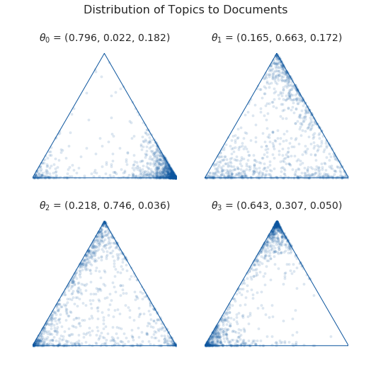
Since we chose to distribute words among three topics, we can examine the distributions of these topics to each document on a simplex. Below, each triangle represents a document and each corner represents a topic. Whenever the sampled points cluster at a corner, that means our model decided that that document was predominantly about the corresponding topic.

with sequence_model:
    pps = pm.sample_posterior_predictive(sequence_trace, vars=[theta], samples=1000, progressbar=False)

var = pps['theta']
thetas = sequence_trace['theta'][4999]
nthetas = thetas.shape[0]

blue = sns.color_palette('Blues_r')[0]
fig = plt.figure()
fig.suptitle('Distribution of Topics to Documents', fontsize=16)
for i, ts in enumerate(thetas):
    plt.subplot(2, nthetas/2, i + 1)
    sp.plot_points(var[:,i], color=blue, marker='o', alpha=0.1, markersize=3)
    title = r'$\theta_{0}$ = ({1[0]:.3f}, {1[1]:.3f}, {1[2]:.3f})'.format(i,ts)
    plt.title(title, fontdict={'fontsize': 14})
random sample of documents in the dirichlet model

That’s all for now!

References

Blei, David M, Andrew Y Ng and Michael I Jordan. 2003. “Latent dirichlet allocation.” Journal of machine Learning research.

https://stackoverflow.com/questions/31473459/pymc3-how-to-implement-latent-dirichlet-allocation

https://github.com/junpenglao/Planet_Sakaar_Data_Science/blob/master/PyMC3QnA/discourse_2314.ipynb