Table of Contents
Imagine we have some collection of documents. They could be novels, or tweets, or financial reports—just any collection of text. We want an algorithm that can discover what they are about, and we would like our algorithm to do it automatically, without any hints. (That is, we want our algorithm to be unsupervised.) We will look at several models that probabilistically assign words to topics using Bayes’ Theorem. They are all Bayesian Graphical Models.
The basic problem in statistics is to infer some unobservable value from observable instances of it. In our case, we want to infer the topics of a document from the actual words in the document. We want to be able to infer that our document is about “colors” if we observe “red” and “green” and “blue”.
Bayes’ Theorem allows us to do this. It allows us to infer probabilities concerning the unobserved value from the observations that we can make. It allows us to reason backwards in some sense. So, when constructing a Bayesian model, it is helpful to think backwards. Instead of first asking how words are distributed to topics and topics to documents, we will ask how we could generate a document if we already knew these distributions. To construct our model, we will first reason from the unknown values to the known values so that we know how to do the converse when the time comes.
Some Simple Generative Examples
In all of our models, we are going make a simplfying assumption. We will assume that all of the words in a document occur independently of whatever words came before or come after; that is, a document will just be a “bag of words.” We’ll see that even with ignoring word-order, we can still infer pretty accurately what a document might be about.
Let’s start with a very simple example: 1 document with 1 topic and 2 words in our vocabulary.
(Some definitions: The “vocabulary” is just the set of unique words that occur in all of the documents together, the “corpus.” We’ll refer to a word in the vocabulary as just a “word” and some instance of a word in a document as a “token.”)
Let’s say our two words are “blue” and “red”, and that the probability of any given word (any token) being “red” is \(\phi\): \(P(W = red) = \phi\). This is the same as saying our random variable of tokens \(W\) has a Bernoulli distribution with parameter \(\phi\): \(W \sim Bernoulli(\phi)\).
The distribution looks like this:
x = [0, 1]
pmf = st.bernoulli.pmf(x, 0.3)

plt.stem(x, pmf)
plt.xticks([0,1])
plt.ylim(0,1)
plt.xlim(-0.5, 1.5)
(-0.5, 1.5)
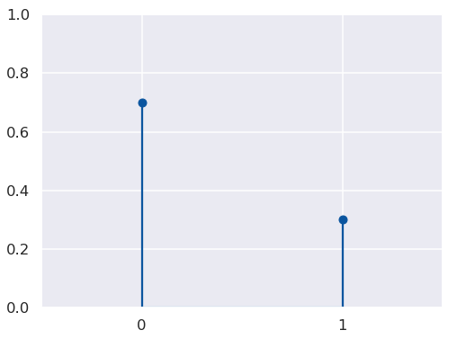
Here, 1 represents “red” and 0 represents “blue” (or not-“red”).
And here is how we could generate a document with this model:
coding = {0 : "blue", 1 : "red"}
W = 50  # number of tokens in the document
tokens = st.bernoulli.rvs(0.3, size = W)  # choose the tokens
print(' '.join(str(w) for w in [coding[i] for i in tokens]))
blue blue red blue red blue blue red red blue blue blue blue blue blue blue blue red blue blue blue blue blue blue blue blue blue red red blue blue blue blue blue blue red blue blue red blue red blue red blue blue blue blue blue red blue
Unigram Model
For the general model, we will also choose the distribution of words within the topic randomly. That is, we will assign a probability distribution to \(\phi\).
The beta distribution is a natural choice. Since its support is \([0,1]\) it can represent randomly chosen probabilities (values between 0 and 1). It is also conceptually convenient being the conjugate prior of the Bernoulli distribution, which allows us to make a more explicit connection between its parameters and the parameters of its Bernoulli distribution.
The model is now:
\(\phi \sim Beta(\beta_0, \beta_1)\)
\(W \sim Bernoulli(\phi)\)
where \(\beta_0\) and \(\beta_1\) are the “shape parameters” of the beta distribution. We can think of them as the assumed counts of each word, or the “pseudo-counts.” Let’s see how different values of these parameters affect the shape of the distribution.
beta_0 = [0.8, 1, 2, 10]
beta_1 = [0.8, 1, 2, 10]

x = np.array(np.linspace(0, 1, 1000))

f, axarr = plt.subplots(len(beta_0), len(beta_1), sharex='all', sharey='none')

for i in range(len(beta_0)):
    for j in range(len(beta_1)):
        a = beta_0[i]
        b = beta_1[j]
        y = st.beta(a, b).pdf(x)
        axarr[i, j].plot(x, y)
        axarr[i, j].axes.yaxis.set_ticklabels([])
        axarr[i, j].set_title(r'$\beta_0 =$ ' + str(a) + r', $\beta_1 =$ ' + str(b))

f.subplots_adjust(hspace=0.3)
f.suptitle(r'Beta Distributions for $\theta$', fontsize=20)
Text(0.5, 0.98, 'Beta Distributions for $\\theta$')
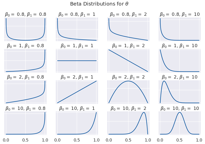
Values near 0 will favor “blue” and values near 1 will favor “red”. We can choose \(\beta_0\) and \(\beta_1\) to generate the kinds of documents we like. (The notation is a bit backwards here: \(\beta_0\) is the pseudo-count for “red”, whose probability is toward 1, on the right of the graph. So \(\beta_0 > \beta_1\) means more “red”s, and vice versa.)
Let’s generate some documents with this expanded model. We’ll set \(\beta_0 = 0.8\) and \(\beta_1 = 0.8\). We would expect most of our documents to favor one word or the other, but overall to occur equally often.
beta_0 = 0.8
beta_1 = 0.8

thetas = st.beta.rvs(beta_0, beta_1, size = 6)

W = 10  # number of tokens in each document

for t in thetas:
    print('Theta: ', t)
    tokens = st.bernoulli.rvs(t, size = W)
    print('Document: ' + ' '.join(str(w) for w in [coding[i] for i in tokens]) + '\n')
Theta:  0.2376299911870814
Document: blue red blue blue red red blue blue blue blue

Theta:  0.768902025579346
Document: red red red red blue red red red blue red

Theta:  0.6339386112711662
Document: red blue red blue red blue blue blue red blue

Theta:  0.889248394241369
Document: red red red blue red red red red red red

Theta:  0.7522981849896823
Document: red red red red blue blue red red red red

Theta:  0.18416659985533126
Document: blue red red blue blue blue red red blue blue
(We could also assign a distribution to W, the number of tokens in each document. (Blei 2003) uses a Poisson distribution.)
Let’s look at a couple more.
Mixture of Unigrams
Here, we’ll also choose a single topic for each document, from among two. To simplify things, we’ll also assume the topics generate distinct words and that the proportions of words in topics are similar, that is, that they have the same shape parameters. We’ll see later that is a good assumption when using inference models.
Distribution of topics to documents: \(\theta \sim Beta(\alpha_0, \alpha_1)\)
Distribution of words to Topic 0: \(\phi_0 \sim Beta(\beta_0, \beta_1)\)
Distribution of words to Topic 1: \(\phi_1 \sim Beta(\beta_0, \beta_1)\)
The topics: \(T \sim Bernoulli(\theta)\)
Words from Topic 0: \(W_1 \sim Bernoulli(\phi_0)\)
Words from Topic 1: \(W_2 \sim Bernoulli(\phi_1)\)
coding_0 = {0:'blue', 1:'red'}  # words in topic 0
coding_1 = {0:'dogs', 1:'cats'}  # words in topic 1

D = 15  # number of documents in corpus
W = 10  # number of tokens in each document

alpha_0, alpha_1 = 1, 1.5
beta_0, beta_1 = 0.8, 0.8

theta = st.beta.rvs(alpha_0, alpha_1, size = 1)[0]  # choose a distribution of topics to documents
phi_0 = st.beta.rvs(beta_0, beta_1, size = 1)[0] # choose distribution of words in topic 0
phi_1 = st.beta.rvs(beta_0, beta_1, size = 1)[0] # choose distribution of words in topic 1

topics = st.bernoulli.rvs(theta, size = D)  # choose a topic for each document

print('Theta: {:.3f}  Phi_0: {:.3f}  Phi_1: {:.3f}'.format(theta, phi_0, phi_1))
for i in range(D):
    if topics[i] == 0:
        tokens = st.bernoulli.rvs(phi_0, size = W)
        print('Document: ' + ' '.join(str(w)
              for w in [coding_0[i] for i in tokens]))
    else:
        tokens = st.bernoulli.rvs(phi_1, size = W)
        print('Document: ' + ' '.join(str(w)
              for w in [coding_1[i] for i in tokens]))
Theta: 0.114  Phi_0: 0.973  Phi_1: 0.637
Document: red red red red red red red red red red
Document: red red red blue red red red red red red
Document: red red red red red red red red red red
Document: red red red red red red red red red red
Document: red red red red red red red red red red
Document: red red red red red red red red red red
Document: red red red red red red red red red red
Document: red red red red red red red red red red
Document: dogs dogs cats cats cats cats cats dogs cats dogs
Document: red red red red red red red red red red
Document: red red red red red red red red red red
Document: red red red red red red red red red red
Document: red red blue red red red red red red red
Document: red red red red red red red red red red
Document: red red red red red red red red red red
Latent Dirichlet Allocation
This time, instead of choosing a single topic for each document, we’ll choose a topic for each word. This will make our model much more flexible and its behavior more realistic.
Distribution of topics within documents: \(\theta \sim Beta(\alpha_0, \alpha_1)\)
Distribution of words to Topic 0: \(\phi_0 \sim Beta(\beta_0, \beta_1)\)
Distribution of words to Topic 1: \(\phi_1 \sim Beta(\beta_0, \beta_1)\)
The topics: \(T \sim Bernoulli(\theta)\)
Words from Topic 0: \(W_1 \sim Bernoulli(\phi_0)\)
Words from Topic 1: \(W_2 \sim Bernoulli(\phi_1)\)
coding_0 = {0:'blue', 1:'red'}  # words in topic 0
coding_1 = {0:'dogs', 1:'cats'}  # words in topic 1

D = 15
W = 10  # number of tokens in each document

alpha_0, alpha_1 = 1, 1.5
beta_0, beta_1 = 0.8, 0.8

theta = st.beta.rvs(alpha_0, alpha_1, size = 1)[0]  # choose a distribution of topics to documents
phi_0 = st.beta.rvs(beta_0, beta_1, size = 1)[0]  # choose distribution of words in topic 0
phi_1 = st.beta.rvs(beta_0, beta_1, size = 1)[0]  # choose distribution of words in topic 1

print('Theta: {:.3f}  Phi_0: {:.3f}  Phi_1: {:.3f}'.format(theta, phi_0, phi_1))
for i in range(D):
    print('Document: ', end='')
    topics = st.bernoulli.rvs(theta, size=W)  # choose topics for each word
    for j in range(W):
        if topics[j] == 0:
            token = st.bernoulli.rvs(phi_0, size=1)[0]  # choose a word from topic 0
            print(coding_0[token], end=' ')
        else:
            token = st.bernoulli.rvs(phi_1, size=1)[0]  # choose a word from topic 1
            print(coding_1[token], end=' ')
    print()
Theta: 0.384  Phi_0: 0.127  Phi_1: 0.028
Document: dogs blue blue blue dogs blue dogs blue blue blue
Document: blue dogs blue blue dogs dogs dogs dogs blue cats
Document: blue dogs blue blue blue dogs red dogs blue blue
Document: dogs dogs red dogs dogs blue dogs blue blue blue
Document: blue dogs dogs blue blue dogs red dogs dogs red
Document: dogs blue blue red dogs blue dogs blue blue blue
Document: blue blue blue dogs blue dogs blue dogs dogs blue
Document: dogs red dogs red dogs blue dogs dogs blue blue
Document: dogs dogs blue dogs blue dogs blue blue blue dogs
Document: dogs blue blue blue blue red blue blue dogs dogs
Document: dogs dogs blue red dogs dogs blue blue blue blue
Document: blue blue blue red dogs blue blue blue blue red
Document: blue blue blue dogs blue dogs red dogs blue dogs
Document: dogs blue blue dogs dogs dogs blue dogs dogs blue
Document: dogs dogs dogs red blue dogs red dogs dogs dogs
The Dirichlet Distribution
Before we go on, we need to generalize our model a bit to be able to handle arbitrary numbers of words and topics, instead of being limited to just two. The multivariate generalization of the Bernoulli distribution is the categorical distribution, which simply gives a probability to each of some number of categories. The generalization of the beta distribution is a little trickier. It is called the Dirichlet distribution. And just like samples from the beta distribution will give parameters for a Bernoulli RV, samples from the Dirichlet distribution will give parameters for the categorical RV.
Let’s recall the two requirements for some set of \(p\)’s to be probability parameters to a categorical distribution. First, they have to sum to 1: \(p_0 + p_1 + \cdots + p_v = 1\). This means they form a hyperplane in \(v\)-dimensional space. Second, they all have to be non-negative: \(p_i \geq 0\). This means they all lie in the first quadrant (or orthant, more precisely). The geometric object that satisfies these two requirements is a simplex. In the case of two variables it will be a line-segment and in the case of three variables it will be a triangle.
As sampled from the distribution, these values will form barycentric coordinates on the simplex. This just means that the coordinates tell you how far the point is from the center of the simplex, instead of how far it is from the origin, like with Cartesian coordinates.
The 3-dimensional Dirichlet returns barycentric coordinates on the 2-simplex, a triangle. We can visualize the surface of the Dirichlet pdf as existing over a triangle; that is, its domain is the simplex.
import simplex_plots as sp
# from https://gist.github.com/tboggs/8778945

alphas = [[0.999, 0.999, 0.999], [1, 2, 1], [1, 2, 3],
          [2, 0.999, 1], [10, 3, 4], [0.999, 1, 1]]

fig = plt.figure(figsize=(12, 8))
fig.suptitle('The Dirichlet Distribution', fontsize=16)
for i, a in enumerate(alphas):
    plt.subplot(2, len(alphas)/2, i + 1)
    sp.draw_pdf_contours(sp.Dirichlet(a), border=True, cmap='Blues')
    title = r'$\alpha = $ = ({0[0]:.3f}, {0[1]:.3f}, {0[2]:.3f})'.format(a)
    plt.title(title, fontdict={'fontsize': 14})
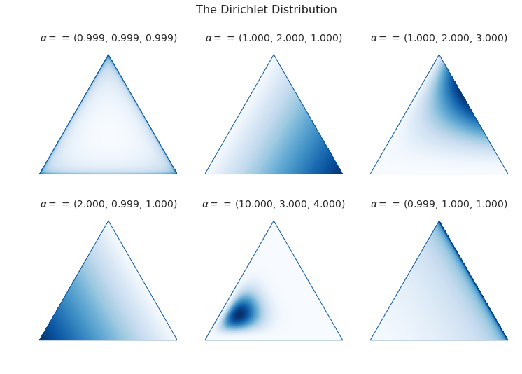
Each corner of the triangle will favor a particular category (a word or a topic), just like either side of the domain of the beta distribution favored a category.
As in the upper left picture, whenever all of the entries in \(\alpha\) are equal, we call the distribution “symmetric,” and whenever they are all less then 1, we call the distribution “sparse.” Distributions that are both symmetric and sparse are often used as priors when inferring a topic model, symmetry because we don’t a priori have any reason to favor one unknown category over another, and sparsity to encourage our categories to be distinct.
Now let’s start developing our models.
The Full Model
Data Preparation
First we’ll make up a corpus and put it into an encoding that our models can use. To simplify things, we’ll let all of our documents have the same number of tokens and flatten the encoded data structure.
from sklearn.preprocessing import LabelEncoder
from sklearn.feature_extraction.text import CountVectorizer

corpus = [
    'Red blue green. Green blue blue? Red, red, blue, yellow.',
    'Car light red stop. Stop car. Car drive green, yellow.',
    'Car engine gas stop! Battery engine drive, car. Electric, gas.',
    'Watt, volt, volt, amp. Battery, watt, volt, electric volt charge. ',
]

tokenizer = CountVectorizer(lowercase=True).build_analyzer()
encoder = LabelEncoder()

corpus_tokenized = np.array([tokenizer(doc) for doc in corpus])  # assign a number to each word
encoder.fit(corpus_tokenized.ravel())
vocab = list(encoder.classes_)  # the vocabulary

# The number of documents and their length
D, W = corpus_tokenized.shape
# The number of words in the vocabulary
V = len(vocab)

# Flatten and encode the corpus, and create an index.
data = corpus_tokenized.ravel()
data = encoder.transform(data)
data_index = np.repeat(np.arange(D), W)
Now a couple of diagnostic functions.
def print_top_words(vocab, phis, n):
    '''Prints the top words occuring within a topic.'''
    for i, p in enumerate(phis):
        z = list(zip(vocab, p))
        z.sort(key = lambda x: x[1], reverse=True)
        z = z[0:n]

        for word, percent in z:
            print(f'Topic: {i:2}  Word: {word:10}  Percent: {percent:0.3f}')

        print()

def print_corpus_topics(corpus_tokenized, zs):
    '''Prints the corpus together with the topic assigned to each word.'''
    for d in range(zs.shape[0]):  # the document index
        for w in range(zs.shape[1]):  # the word index
            print(f'({corpus_tokenized[d, w]}, {zs[d, w]})', end=' ')
        print('\n')
The Unigram Model
In this model, words from every document are drawn from a single categorical distribution.
Distribution of words in a document: \(\phi \sim Dir(\vec{\beta})\), where \(\vec{\beta}\) is a vector of shape parameters
Distribution of tokens: \(W \sim Cat(\vec{\phi})\)
Markov-Chain Monte Carlo is a technique for sampling a model to discover its posterior parameters statistically. When models become complex, it is often the case that analytic solutions for the parameters are intractable. We will use the PyMC3 package.
First we describe the model.
# Pseudo-counts for each vocab word occuring in the documents.
beta = np.ones(V)

with pm.Model() as unigram_model:

    # Distribution of word-types in the corpus.
    phi = pm.Dirichlet('phi', a = beta)

    # The distribution of words.
    w = pm.Categorical('w', p = phi, observed = data)
Next we sample the model to create the posterior distribution.
with unigram_model:
    draw = 5000
    unigram_trace = pm.sample(5000, tune=1000, chains=4, progressbar=False)
And now we can see what the model determined the proportion of each word in the corpus was.
print_top_words(vocab, [unigram_trace.get_values('phi')[draw-1]], len(vocab))
Topic:  0  Word: red         Percent: 0.150
Topic:  0  Word: watt        Percent: 0.145
Topic:  0  Word: car         Percent: 0.117
Topic:  0  Word: green       Percent: 0.080
Topic:  0  Word: battery     Percent: 0.073
Topic:  0  Word: volt        Percent: 0.068
Topic:  0  Word: yellow      Percent: 0.067
Topic:  0  Word: drive       Percent: 0.059
Topic:  0  Word: electric    Percent: 0.054
Topic:  0  Word: gas         Percent: 0.053
Topic:  0  Word: stop        Percent: 0.048
Topic:  0  Word: blue        Percent: 0.030
Topic:  0  Word: engine      Percent: 0.025
Topic:  0  Word: charge      Percent: 0.021
Topic:  0  Word: light       Percent: 0.011
Topic:  0  Word: amp         Percent: 0.002
Mixture of Unigrams (Naive Bayes)
In this model, each document is assigned a topic and each topic has its own distribution of words.
Distribution of topics to documents: \(\vec{\theta} \sim Dirichlet(\vec{\alpha})\)
Distribution of words to topics: \(\vec{\phi} \sim Dirichlet(\vec{\beta})\)
The topics: \(T \sim Categorical(\vec{\theta})\)
The tokens: \(W \sim Categorical(\vec{\phi})\)
# Number of topics
K = 3

# Pseudo-counts for topics and words.
alpha = np.ones(K)*0.8
beta = np.ones(V)*0.8

with pm.Model() as naive_model:
    # Global topic distribution
    theta = pm.Dirichlet("theta", a=alpha)

    # Word distributions for K topics
    phi = pm.Dirichlet("phi", a=beta, shape=(K, V))

    # Topic of documents
    z = pm.Categorical("z", p=theta, shape=D)

    # Words in documents
    p = phi[z][data_index]
    w = pm.Categorical("w", p=p, observed=data)
with naive_model:
    draw = 5000
    naive_trace = pm.sample(draw, tune=1000, chains=4, progressbar=False)
print_top_words(vocab, naive_trace['phi'][draw-1], 5)
Topic:  0  Word: drive       Percent: 0.177
Topic:  0  Word: car         Percent: 0.166
Topic:  0  Word: red         Percent: 0.126
Topic:  0  Word: blue        Percent: 0.108
Topic:  0  Word: green       Percent: 0.086

Topic:  1  Word: car         Percent: 0.238
Topic:  1  Word: green       Percent: 0.192
Topic:  1  Word: watt        Percent: 0.180
Topic:  1  Word: blue        Percent: 0.070
Topic:  1  Word: red         Percent: 0.045

Topic:  2  Word: volt        Percent: 0.161
Topic:  2  Word: car         Percent: 0.123
Topic:  2  Word: engine      Percent: 0.113
Topic:  2  Word: electric    Percent: 0.094
Topic:  2  Word: gas         Percent: 0.081
Latent Dirichlet Allocation
In this model, each word is assigned a topic and topics are distributed varyingly within each document.
Distribution of topics within documents: \(\vec{\theta} \sim Dirichlet(\vec{\alpha})\)
Distribution of words to topics: \(\vec{\phi} \sim Dirichlet(\vec{\beta})\)
The topics: \(T \sim Categorical(\vec{\theta})\)
The tokens: \(W \sim Categorical(\vec{\phi})\)
# Number of topics
K = 3

# Pseudo-counts. Sparse to encourage separation.
alpha = np.ones((1, K))*0.5
beta = np.ones((1, V))*0.5

with pm.Model() as lda_model:
    # Distribution of topics within each document
    theta = pm.Dirichlet("theta", a=alpha, shape=(D, K))

    # Distribution of words within each topic
    phi = pm.Dirichlet("phi", a=beta, shape=(K, V))

    # The topic for each word
    z = pm.Categorical("z", p=theta, shape=(W, D))

    # Words in documents
    p = phi[z].reshape((D*W, V))
    w = pm.Categorical("w", p=p, observed=data)
with lda_model:
    draw = 5000
    lda_trace = pm.sample(draw, tune=1000, chains=4, progressbar=False)

print_top_words(tokens, lda_trace.get_values('phi')[draw-1], 4)
At the cost of some complexity, we can rewrite our model to handle a corpus with documents of varying lengths.
alpha = np.ones([D, K])*0.5  # prior weights for the topics in each document (pseudo-counts)
beta  = np.ones([K, V])*0.5  # prior weights for the vocab words in each topic (pseudo-counts)

sequence_data = np.reshape(np.array(data), (D,W))
N = np.repeat(W, D)  # this model needs a list of document lengths

with pm.Model() as sequence_model:

    # distribution of the topics occuring in a particular document
    theta   = pm.Dirichlet('theta', a=alpha, shape=(D, K))

    # distribution of the vocab words occuring in a particular topic
    phi     = pm.Dirichlet('phi', a=beta, shape=(K, V))

    # the topic for a particular word in a particular document: shape = (D, N[d])
    # theta[d] is the vector of category probabilities for each topic in
    # document d.
    z = [pm.Categorical('z_{}'.format(d), p = theta[d], shape=N[d])
          for d in range(D)]

    # the word occuring at position n, in a particular document d: shape = (D, N[d])
    # z[d] is the vector of topics for document d
    # z[d][n] is the topic for word n in document d
    # phi[z[d][n]] is the distribution of words for topic z[d][n]
    # [d][n] is the n-th word observed in document d
    w = [pm.Categorical('w_{}_{}'.format(d, n), p=phi[z[d][n]],
                        observed = sequence_data[d][n])
         for d in range(D) for n in range(N[d])]

with sequence_model:
    draw = 5000
    sequence_trace = pm.sample(draw, tune=1000, chains=4, progressbar=False)

print_top_words(tokens, sequence_trace.get_values('phi')[4999], 4)
And here we can see what topic the model assigned to each token in the corpus.
zs = [sequence_trace.get_values('z_{}'.format(d))[draw-1] for d in range(D)]
zs = np.array(zs)

print_corpus_topics(corpus_tokenized, zs)
(red, 2) (blue, 0) (green, 0) (green, 0) (blue, 0) (blue, 0) (red, 2) (red, 0) (blue, 0) (yellow, 0)

(car, 1) (light, 2) (red, 1) (stop, 1) (stop, 1) (car, 1) (car, 1) (drive, 1) (green, 2) (yellow, 1)

(car, 1) (engine, 1) (gas, 1) (stop, 1) (battery, 1) (engine, 1) (drive, 1) (car, 0) (electric, 1) (gas, 1)

(watt, 0) (volt, 0) (volt, 0) (amp, 1) (battery, 1) (watt, 0) (volt, 0) (electric, 0) (volt, 0) (charge, 0)
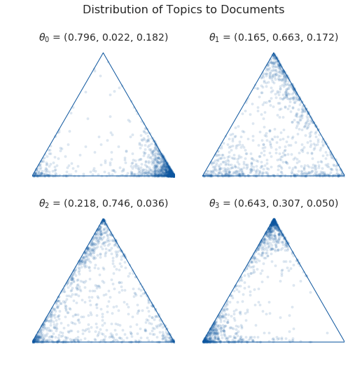
Since we chose to distribute words among three topics, we can examine the distributions of these topics to each document on a simplex. Below, each triangle represents a document and each corner represents a topic. Whenever the sampled points cluster at a corner, that means our model decided that that document was predominantly about the corresponding topic.
with sequence_model:
    pps = pm.sample_posterior_predictive(sequence_trace, vars=[theta], samples=1000, progressbar=False)

var = pps['theta']
thetas = sequence_trace['theta'][4999]
nthetas = thetas.shape[0]

blue = sns.color_palette('Blues_r')[0]
fig = plt.figure()
fig.suptitle('Distribution of Topics to Documents', fontsize=16)
for i, ts in enumerate(thetas):
    plt.subplot(2, nthetas/2, i + 1)
    sp.plot_points(var[:,i], color=blue, marker='o', alpha=0.1, markersize=3)
    title = r'$\theta_{0}$ = ({1[0]:.3f}, {1[1]:.3f}, {1[2]:.3f})'.format(i,ts)
    plt.title(title, fontdict={'fontsize': 14})
That’s all for now!
References
Blei, David M, Andrew Y Ng and Michael I Jordan. 2003. “Latent dirichlet allocation.” Journal of machine Learning research.
https://stackoverflow.com/questions/31473459/pymc3-how-to-implement-latent-dirichlet-allocation
https://github.com/junpenglao/Planet_Sakaar_Data_Science/blob/master/PyMC3QnA/discourse_2314.ipynb
Comments powered by Talkyard.